Tutorial

Authors: Pierre-Henri Tournier - Frédéric Nataf - Pierre Jolivet

We recommend checking the slides version of this tutorial.

What is ffddm ?

ffddm implements a class of parallel solvers in FreeFEM: overlapping Schwarz domain decomposition methods
The entire ffddm framework is written in the FreeFEM language ffddm aims at simplifying the use of parallel solvers in FreeFEM
You can find the ffddm scripts here (‘ffddm*.idp’ files) and examples here
ffddm provides a set of high-level macros and functions to
- handle data distribution: distributed meshes and linear algebra
- build DD preconditioners for your variational problems
- solve your problem using preconditioned Krylov methods
ffddm implements scalable two level Schwarz methods, with a coarse space correction built either from a coarse mesh or a GenEO coarse space Ongoing research: approximate coarse solves and three level methods
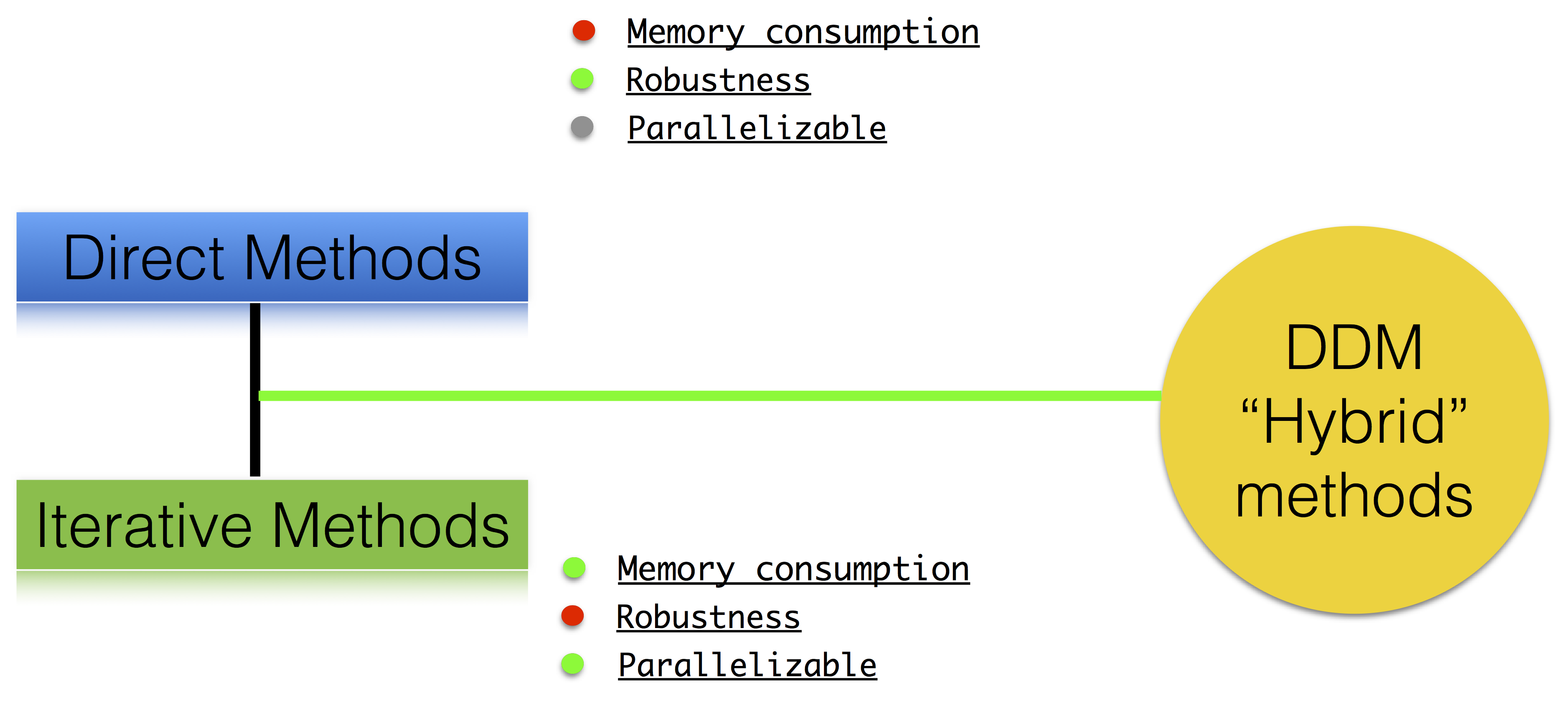
ffddm can also act as a wrapper for the HPDDM library.
HPDDM is an efficient C++11 implementation of various domain decomposition methods and Krylov subspace algorithms with advanced block and recycling techniques More details on how to use HPDDM within ffddm here

Why Domain Decomposition Methods ?

How can we solve a large sparse linear system $A u = b \in \mathbb{R}^n$ ?

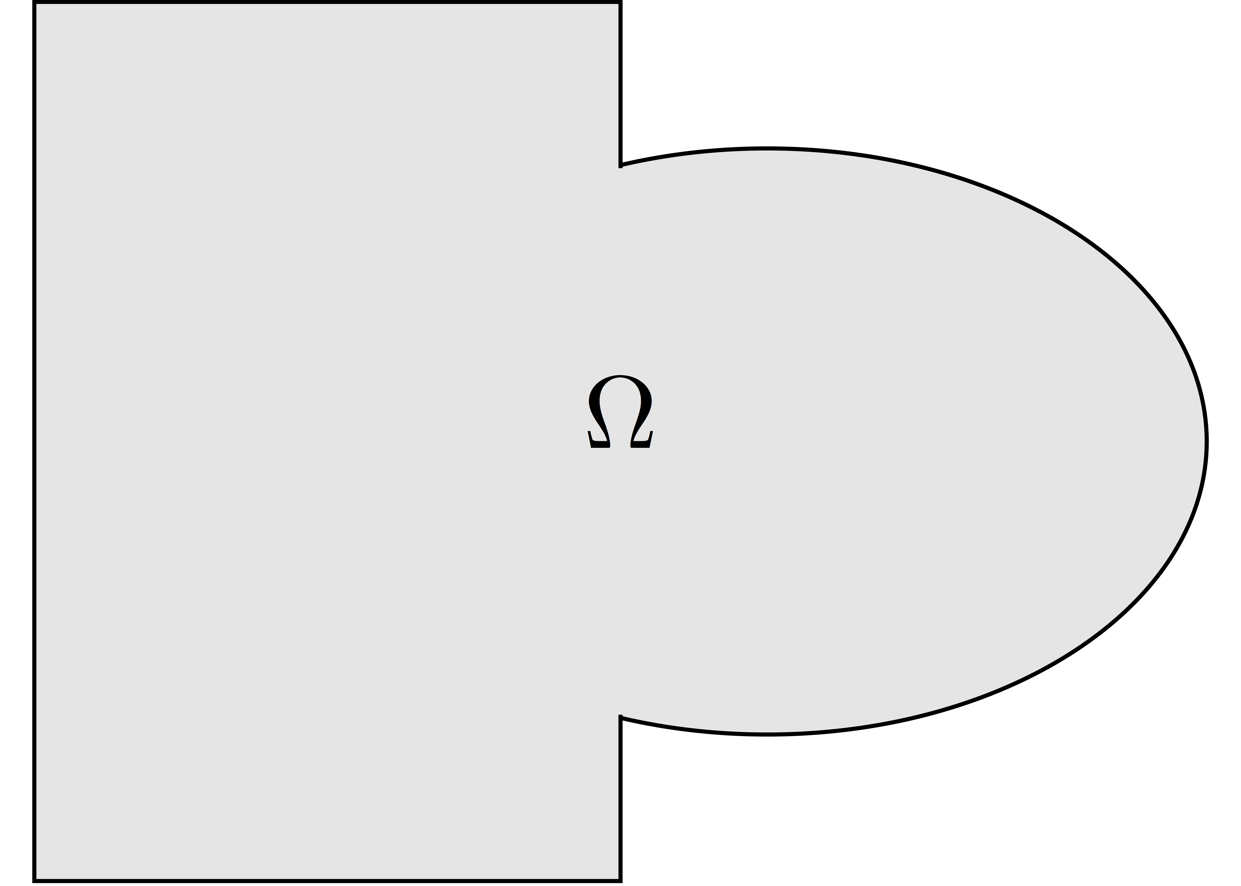
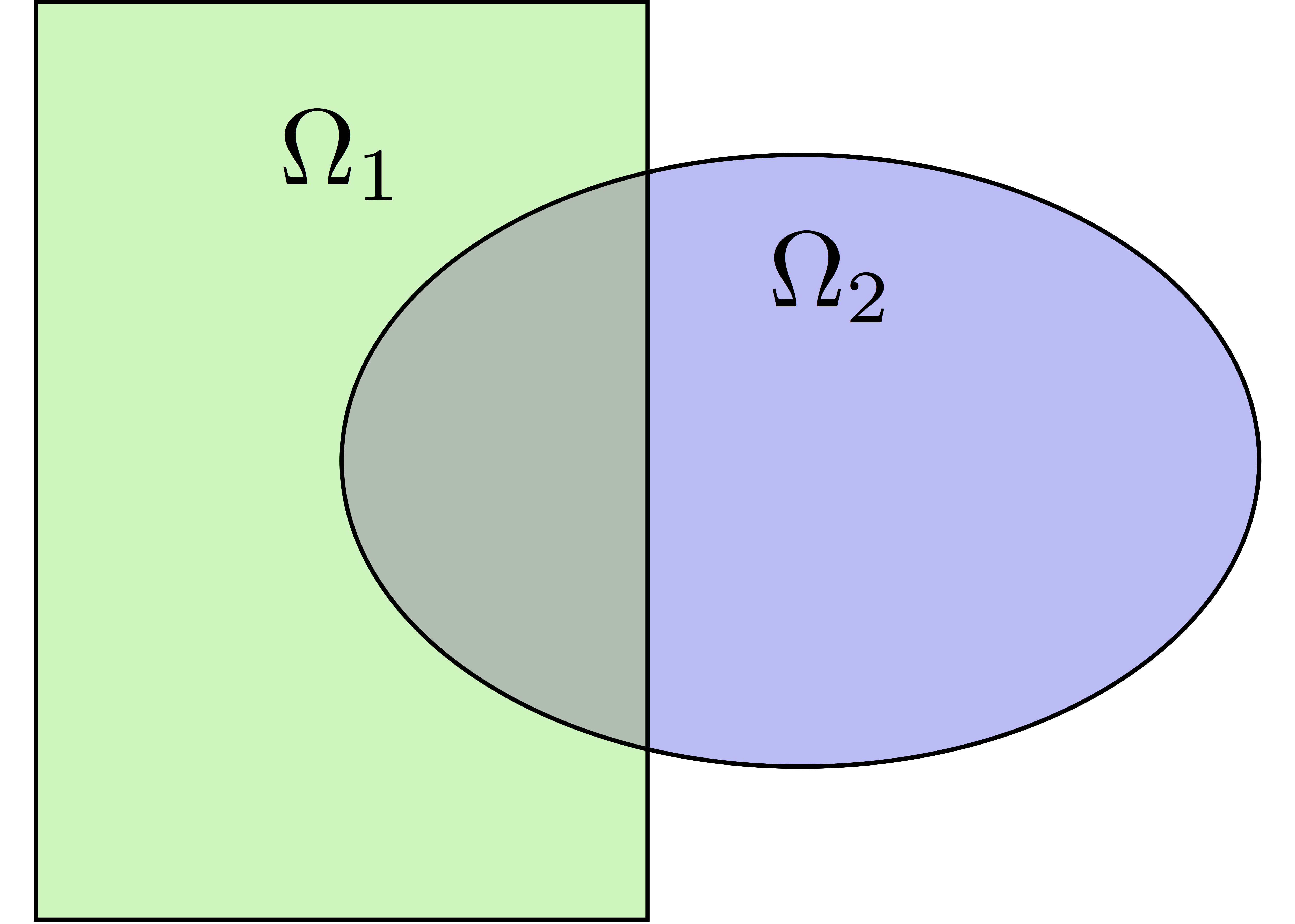
Step 1: Decompose the mesh

See documentation

Build a collection of $N$ overlapping sub-meshes $(Th_{i})_{i=1}^N$ from the global mesh $Th$

ffddmbuildDmesh( prmesh , ThGlobal , comm )

mesh distributed over the MPI processes of communicator comm
initial mesh ThGlobal partitioned with metis by default
size of the overlap given by ffddmoverlap (default 1)

prmesh#Thi is the local mesh of the subdomain for each mpi process

macro dimension 2// EOM            // 2D or 3D

include "ffddm.idp"

mesh ThGlobal = square(100,100);    // global mesh

// Step 1: Decompose the mesh
ffddmbuildDmesh( M , ThGlobal , mpiCommWorld )

medit("Th"+mpirank, MThi);

Copy and paste this to a file ‘test.edp’ and run it:

ff-mpirun -np 2 test.edp -wg

Step 2: Define your finite element

See documentation

ffddmbuildDfespace( prfe , prmesh , scalar , def , init , Pk )

builds the local finite element spaces and associated distributed operators on top of the mesh decomposition prmesh

scalar: type of data for this finite element: real or complex
Pk: your type of finite element: P1, [P2,P2,P1], …
def, init: macros specifying how to define and initialize a Pk FE function

prfe#Vhi is the local FE space defined on prmesh#Thi for each mpi process

Example for P2 complex:

macro def(u)  u // EOM
macro init(u) u // EOM
ffddmbuildDfespace( FE, M, complex,
                    def, init, P2 )

Example for [P2,P2,P1] real:

macro def(u)  [u, u#B, u#C] // EOM
macro init(u) [u, u, u]     // EOM
ffddmbuildDfespace( FE, M, real, def,
                    init, [P2,P2,P1] )

Distributed vectors and restriction operators

Natural decomposition of the set of d.o.f.’s ${\mathcal N}$ of $Vh$ into the $N$ subsets of d.o.f.’s $({\mathcal N}_i)_{i=1}^N$ each associated with the local FE space $Vh_i$

\[{\mathcal N} = \cup_{i=1}^N {\mathcal N}_i\,,\]

but with duplications of the d.o.f.’s in the overlap

_Definition_ a distributed vector is a collection of local vectors $({\mathbf V_i})_{1\le i\le N}$ so that the values on the duplicated d.o.f.’s are the same:

\[{\mathbf V}_i = R_i\,{\mathbf V}, \quad i = 1, ..., N\]

where ${\mathbf V}$ is the corresponding global vector and $R_i$ is the restriction operator from ${\mathcal N}$ into ${\mathcal N}_i$

Remark $R_i^T$ is the extension operator: extension by $0$ from ${\mathcal N}_i$ into ${\mathcal N}$

Partition of unity

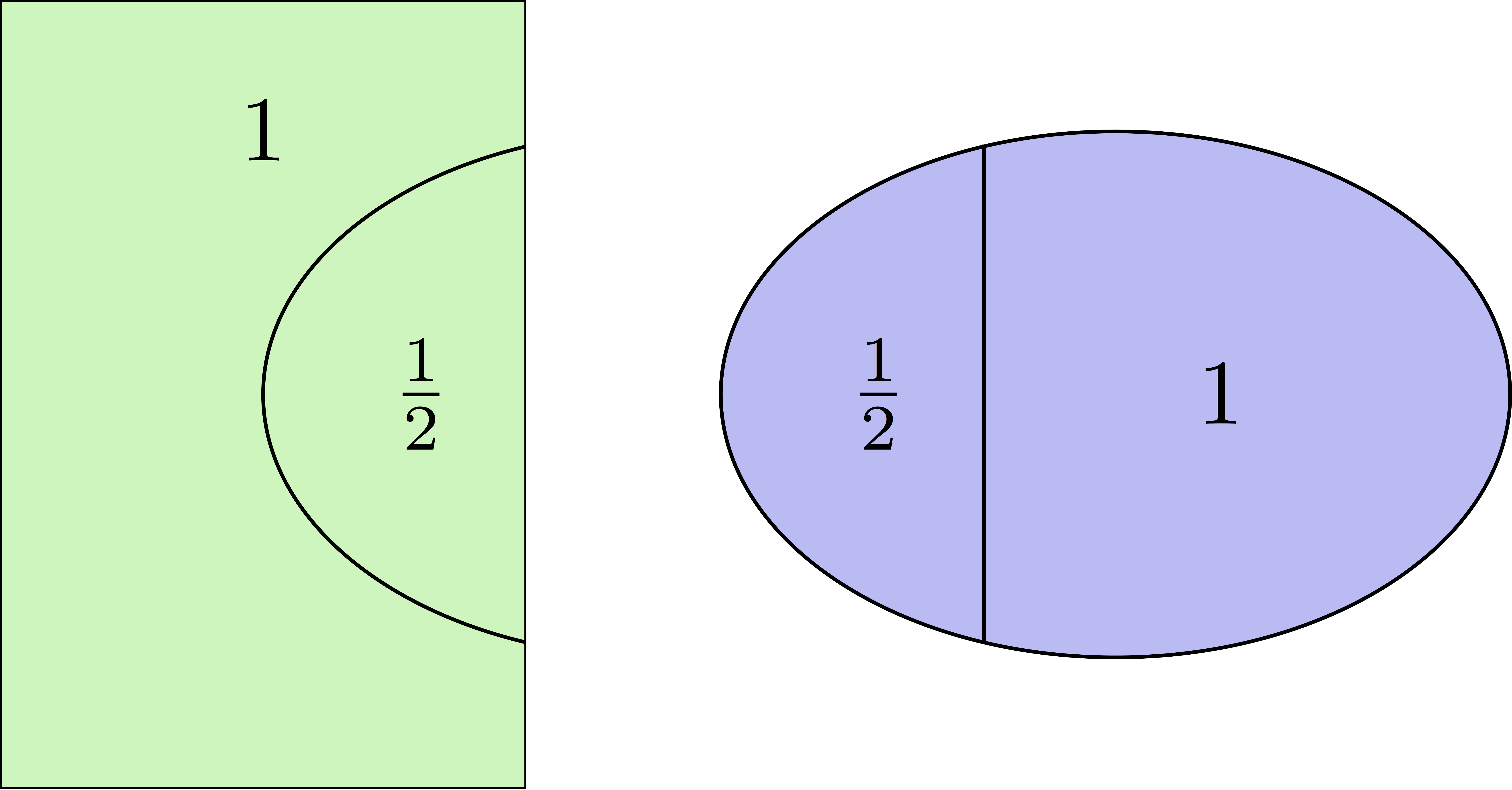
Duplicated unknowns coupled via a partition of unity:

\[I = \sum_{i = 1}^N R_i^T D_i R_i\]

$(D_i)_{1\le i \le N}$ are square diagonal matrices of size $\#{\mathcal N}_i$

\[{\mathbf V} = \sum_{i = 1}^N R_i^T D_i R_i {\mathbf V} = \sum_{i = 1}^N R_i^T D_i {\mathbf V_i}\]

Data exchange between neighbors

func prfe#update(K[int] vi, bool scale)

synchronizes local vectors ${\mathbf V}_i$ between subdomains $\Rightarrow$ exchange the values of $mathbf{V}_i$ shared with neighbors in the overlap region

\[{\mathbf V}_i \leftarrow R_i \left( \sum_{j=1}^N R_j^T D_j {\mathbf V}_j \right) = D_i {\mathbf V}_i + \sum_{j\in \mathcal{O}(i)} R_i\,R_j^T\,D_j {\mathbf V}_j\]

where $\mathcal{O}(i)$ is the set of neighbors of subdomain $i$. Exchange operators $R_i\,R_j^T$ correspond to neighbor-to-neighbor MPI communications

FEupdate(vi, false);

\[{\mathbf V}_i \leftarrow R_i \left( \sum_{j=1}^N R_j^T {\mathbf V}_j \right)\]

FEupdate(vi, true);

\[{\mathbf V}_i \leftarrow R_i \left( \sum_{j=1}^N R_j^T D_j {\mathbf V}_j \right)\]

macro dimension 2// EOM            // 2D or 3D

include "ffddm.idp"

mesh ThGlobal = square(100,100);    // global mesh

// Step 1: Decompose the mesh
ffddmbuildDmesh( M , ThGlobal , mpiCommWorld )

// Step 2: Define your finite element
macro def(u)  u // EOM
macro init(u) u // EOM
ffddmbuildDfespace( FE , M , real , def , init , P2 )

FEVhi vi = x;
medit("v"+mpirank, MThi, vi);

vi[] = FEDk[mpirank];
medit("D"+mpirank, MThi, vi);

vi = 1;
FEupdate(vi[],true);
ffddmplot(FE,vi,"1")

FEupdate(vi[],false);
ffddmplot(FE,vi,"multiplicity")

Step 3: Define your problem

See documentation

ffddmsetupOperator( pr , prfe , Varf )

builds the distributed operator associated to your variational form on top of the distributed FE prfe

Varf is a macro defining your abstract variational form

macro Varf(varfName, meshName, VhName)
    varf varfName(u,v) = int2d(meshName)(grad(u)'* grad(v))
                       + int2d(meshName)(f*v) + on(1, u = 0);  // EOM

$\Rightarrow$ assemble local ‘Dirichlet’ matrices $A_i = R_i A R_i^T$

\[A = \sum_{i=1}^N R_i^T D_i A_i R_i\]

Warning

only true because $D_i R_i A = D_i A_i R_i$ due to the fact that $D_i$ vanishes at the interface !!

pr#A applies $A$ to a distributed vector: ${\mathbf U}_i \leftarrow R_i \sum_{j=1}^N R_j^T D_j A_j {\mathbf V}_j$

$\Rightarrow$ multiply by $A_i$ + prfe#update

macro dimension 2// EOM            // 2D or 3D

include "ffddm.idp"

mesh ThGlobal = square(100,100);    // global mesh

// Step 1: Decompose the mesh
ffddmbuildDmesh( M , ThGlobal , mpiCommWorld )

// Step 2: Define your finite element
macro def(u)  u // EOM
macro init(u) u // EOM
ffddmbuildDfespace( FE , M , real , def , init , P2 )

// Step 3: Define your problem
macro grad(u) [dx(u), dy(u)] // EOM
macro Varf(varfName, meshName, VhName)
    varf varfName(u,v) = int2d(meshName)(grad(u)'* grad(v))
                       + int2d(meshName)(1*v) + on(1, u = 0);  // EOM
ffddmsetupOperator( PB , FE , Varf )

FEVhi ui, bi;
ffddmbuildrhs( PB , Varf , bi[] )

ui[] = PBA(bi[]);
ffddmplot(FE, ui, "A*b")

Summary so far: translating your sequential FreeFEM script

Step 1: Decompose the mesh

See documentation

mesh Th = square(100,100);

mesh Th = square(100,100);
ffddmbuildDmesh(M, Th, mpiCommWorld)

Step 2: Define your finite element

See documentation

fespace Vh(Th, P1);

macro def(u)  u // EOM
macro init(u) u // EOM
ffddmbuildDfespace(FE, M, real, def, init, P1)

Step 3: Define your problem

See documentation

varf Pb(u, v) = ...
matrix A = Pb(Vh, Vh);

macro Varf(varfName, meshName, VhName)
    varf varfName(u,v) = ... // EOM
ffddmsetupOperator(PB, FE, Varf)

Solve the linear system

See documentation

u[] = A^-1 * b[];

ui[] = PBdirectsolve(bi[]);

Solve the linear system with the parallel direct solver MUMPS

See documentation

func K[int] pr#directsolve(K[int]& bi)

We have $A$ and $b$ in distributed form, we can solve the linear system $A u = b$ using the parallel direct solver MUMPS

// Solve the problem using the direct parallel solver MUMPS
ui[] = PBdirectsolve(bi[]);
ffddmplot(FE, ui, "u")

Step 4: Define the one level DD preconditioner

See documentation

ffddmsetupPrecond( pr , VarfPrec )

builds the one level preconditioner for problem pr.

By default it is the Restricted Additive Schwarz (RAS) preconditioner:

\[M^{-1}_1 = M^{-1}_{\text{RAS}} = \sum_{i=1}^N R_i^T D_i A_i^{-1} R_i \quad \text{with}\; A_i = R_i A R_i^T\]

_Setup step_: compute the $LU$ (or $L D L^T$) factorization of local matrices $A_i$

pr#PREC1 applies $M^{-1}_1$ to a distributed vector: ${\mathbf U}_i \leftarrow R_i \sum_{j=1}^N R_j^T D_j A_j^{-1} {\mathbf V}_i$

$\Rightarrow$ apply $A_i^{-1}$ (forward/backward substitutions) + prfe#update

Step 5: Solve the linear system with preconditioned GMRES

See documentation

func K[int] pr#fGMRES(K[int]& x0i, K[int]& bi, real eps, int itmax, string sp)

solves the linear system with flexible GMRES with DD preconditioner $M^{-1}$

x0i: initial guess
bi: right-hand side
eps: relative tolerance
itmax: maximum number of iterations
sp: “left” or “right” preconditioning

left preconditioning

solve $M^{-1} A x = M^{-1} b$

right preconditioning

solve $A M^{-1} y = b$

$\Rightarrow x = M^{-1} y$

macro dimension 2// EOM            // 2D or 3D
include "ffddm.idp"

mesh ThGlobal = square(100,100);    // global mesh
// Step 1: Decompose the mesh
ffddmbuildDmesh( M , ThGlobal , mpiCommWorld )
// Step 2: Define your finite element
macro def(u)  u // EOM
macro init(u) u // EOM
ffddmbuildDfespace( FE , M , real , def , init , P2 )
// Step 3: Define your problem
macro grad(u) [dx(u), dy(u)] // EOM
macro Varf(varfName, meshName, VhName)
    varf varfName(u,v) = int2d(meshName)(grad(u)'* grad(v))
                       + int2d(meshName)(1*v) + on(1, u = 0);  // EOM
ffddmsetupOperator( PB , FE , Varf )

FEVhi ui, bi;
ffddmbuildrhs( PB , Varf , bi[] )

// Step 4: Define the one level DD preconditioner
ffddmsetupPrecond( PB , Varf )

// Step 5: Solve the linear system with GMRES
FEVhi x0i = 0;
ui[] = PBfGMRES(x0i[], bi[], 1.e-6, 200, "right");

ffddmplot(FE, ui, "u")
PBwritesummary

Define a two level DD preconditioner

See documentation

Goal improve scalability of the one level method

$\Rightarrow$ enrich the one level preconditioner with a coarse problem coupling all subdomains

Main ingredient is a rectangular matrix $\color{red}{Z}$ of size $n \times n_c,\,$ where $n_c \ll n$ $\color{red}{Z}$ is the coarse space matrix

The coarse space operator $E = \color{red}{Z}^T A \color{red}{Z}$ is a square matrix of size $n_c \times n_c$

The simplest way to enrich the one level preconditioner is through the additive coarse correction formula:

\[M^{-1}_2 = M^{-1}_1 + \color{red}{Z} E^{-1} \color{red}{Z}^T\]

How to choose $\color{red}{Z}$ ?

Build the GenEO coarse space

See documentation

ffddmgeneosetup( pr , Varf )

The GenEO method builds a robust coarse space for highly heterogeneous or anisotropic SPD problems

$\Rightarrow$ solve a local generalized eigenvalue problem in each subdomain

\[D_i A_i D_i\, V_{i,k} = \lambda_{i,k}\, A_i^{\text{Neu}} \,V_{i,k}\]

with $A_i^{\text{Neu}}$ the local Neumann matrices built from Varf (same Varf as Step 3)

The GenEO coarse space is $\color{red}{Z} = (R_i^T D_i V_{i,k})^{i=1,...,N}_{\lambda_{i,k} \ge \color{blue}{\tau}}$ The eigenvectors $V_{i,k}$ selected to enter the coarse space correspond to eigenvalues $\lambda_{i,k} \ge \color{blue}{\tau}$, where $\color{blue}{\tau}$ is a threshold parameter

Theorem the spectrum of the preconditioned operator lies in the interval $[\displaystyle \frac{1}{1+k_1 \color{blue}{\tau}} , k_0 ]$ where $k_0 - 1$ is the # of neighbors and $k_1$ is the multiplicity of intersections $\Rightarrow$ $k_0$ and $k_1$ do not depend on $N$ nor on the PDE

macro dimension 2// EOM            // 2D or 3D
include "ffddm.idp"

mesh ThGlobal = square(100,100);    // global mesh
// Step 1: Decompose the mesh
ffddmbuildDmesh( M , ThGlobal , mpiCommWorld )
// Step 2: Define your finite element
macro def(u)  u // EOM
macro init(u) u // EOM
ffddmbuildDfespace( FE , M , real , def , init , P2 )
// Step 3: Define your problem
macro grad(u) [dx(u), dy(u)] // EOM
macro Varf(varfName, meshName, VhName)
    varf varfName(u,v) = int2d(meshName)(grad(u)'* grad(v))
                       + int2d(meshName)(1*v) + on(1, u = 0);  // EOM
ffddmsetupOperator( PB , FE , Varf )

FEVhi ui, bi;
ffddmbuildrhs( PB , Varf , bi[] )

// Step 4: Define the one level DD preconditioner
ffddmsetupPrecond( PB , Varf )

// Build the GenEO coarse space
ffddmgeneosetup( PB , Varf )

// Step 5: Solve the linear system with GMRES
FEVhi x0i = 0;
ui[] = PBfGMRES(x0i[], bi[], 1.e-6, 200, "right");

Build the coarse space from a coarse mesh

See documentation

ffddmcoarsemeshsetup( pr , Thc , VarfEprec , VarfAprec )

For non SPD problems, an alternative is to build the coarse space by discretizing the PDE on a coarser mesh Thc

$Z$ will be the interpolation matrix from the coarse FE space ${Vh}_c$ to the original FE space $Vh$

$\Rightarrow E=\color{red}{Z}^{T} A \color{red}{Z}$ is the matrix of the problem discretized on the coarse mesh

The variational problem to be discretized on Thc is given by macro VarfEprec

VarfEprec can differ from the original Varf of the problem

Example: added absorption for wave propagation problems

Similarly, VarfAprec specifies the global operator involved in multiplicative coarse correction formulas. It defaults to $A$ if VarfAprec is not defined

macro dimension 2// EOM            // 2D or 3D
include "ffddm.idp"

mesh ThGlobal = square(100,100);    // global mesh
// Step 1: Decompose the mesh
ffddmbuildDmesh( M , ThGlobal , mpiCommWorld )
// Step 2: Define your finite element
macro def(u)  u // EOM
macro init(u) u // EOM
ffddmbuildDfespace( FE , M , real , def , init , P2 )
// Step 3: Define your problem
macro grad(u) [dx(u), dy(u)] // EOM
macro Varf(varfName, meshName, VhName)
    varf varfName(u,v) = int2d(meshName)(grad(u)'* grad(v))
                       + int2d(meshName)(1*v) + on(1, u = 0);  // EOM
ffddmsetupOperator( PB , FE , Varf )

FEVhi ui, bi;
ffddmbuildrhs( PB , Varf , bi[] )

// Step 4: Define the one level DD preconditioner
ffddmsetupPrecond( PB , Varf )

// Build the coarse space from a coarse mesh
mesh Thc = square(10,10);
ffddmcoarsemeshsetup( PB , Thc , Varf , null )

// Step 5: Solve the linear system with GMRES
FEVhi x0i = 0;
ui[] = PBfGMRES(x0i[], bi[], 1.e-6, 200, "right");

Use HPDDM within ffddm

See documentation

ffddm allows you to use HPDDM to solve your problem, effectively replacing the ffddm implementation of all parallel linear algebra computations

$\Rightarrow$ define your problem with ffddm, solve it with HPDDM

$\Rightarrow$ ffddm acts as a finite element interface for HPDDM

You can use HPDDM features unavailable in ffddm such as advanced Krylov subspace methods implementing block and recycling techniques

To switch to HPDDM, simply define the macro pr#withhpddm before using ffddmsetupOperator (Step 3). You can then pass HPDDM options with command-line arguments or directly to the underlying HPDDM operator. Options need to be prefixed by the operator prefix:

macro PBwithhpddm()1 // EOM
ffddmsetupOperator( PB , FE , Varf )
set(PBhpddmOP,sparams="-hpddm_PB_krylov_method gcrodr -hpddm_PB_recycle 10");

Or, define pr#withhpddmkrylov to use HPDDM only for the Krylov method

Example here: Helmholtz problem with multiple rhs solved with Block GMRES

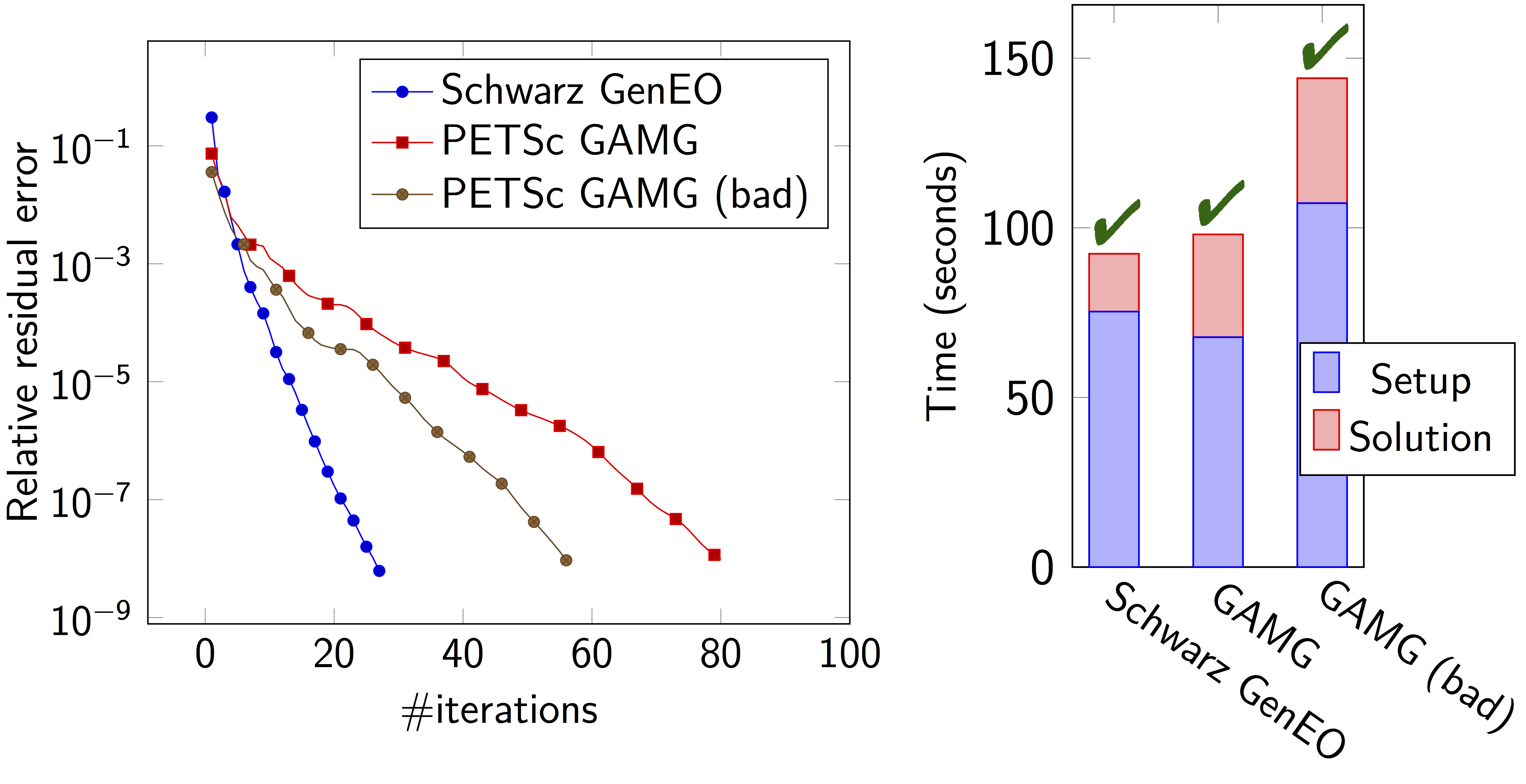
Some results: Heterogeneous 3D elasticity with GenEO

Heterogeneous 3D linear elasticity equation discretized with P2 FE solved on 4096 MPI processes $n\approx$ 262 million

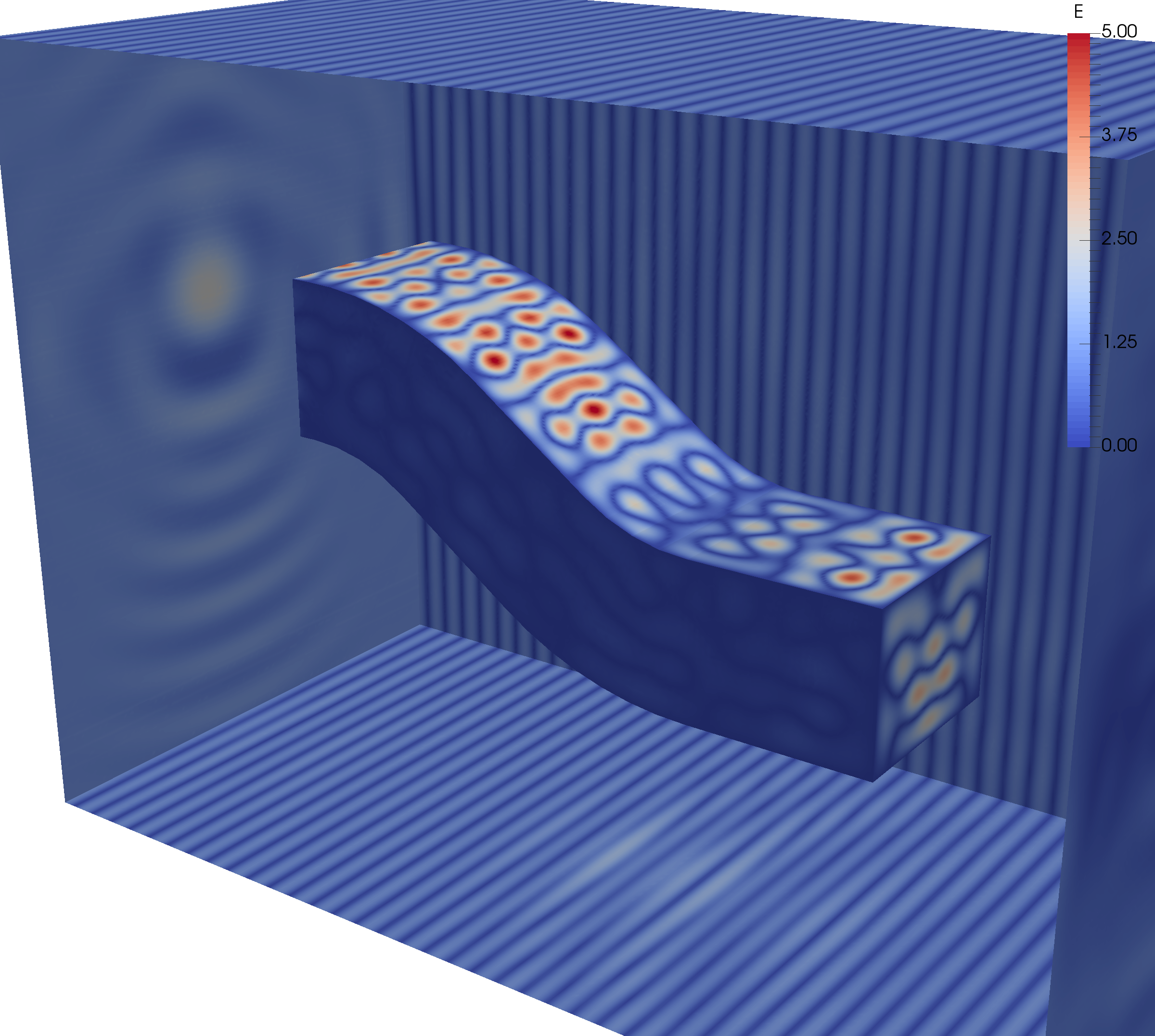
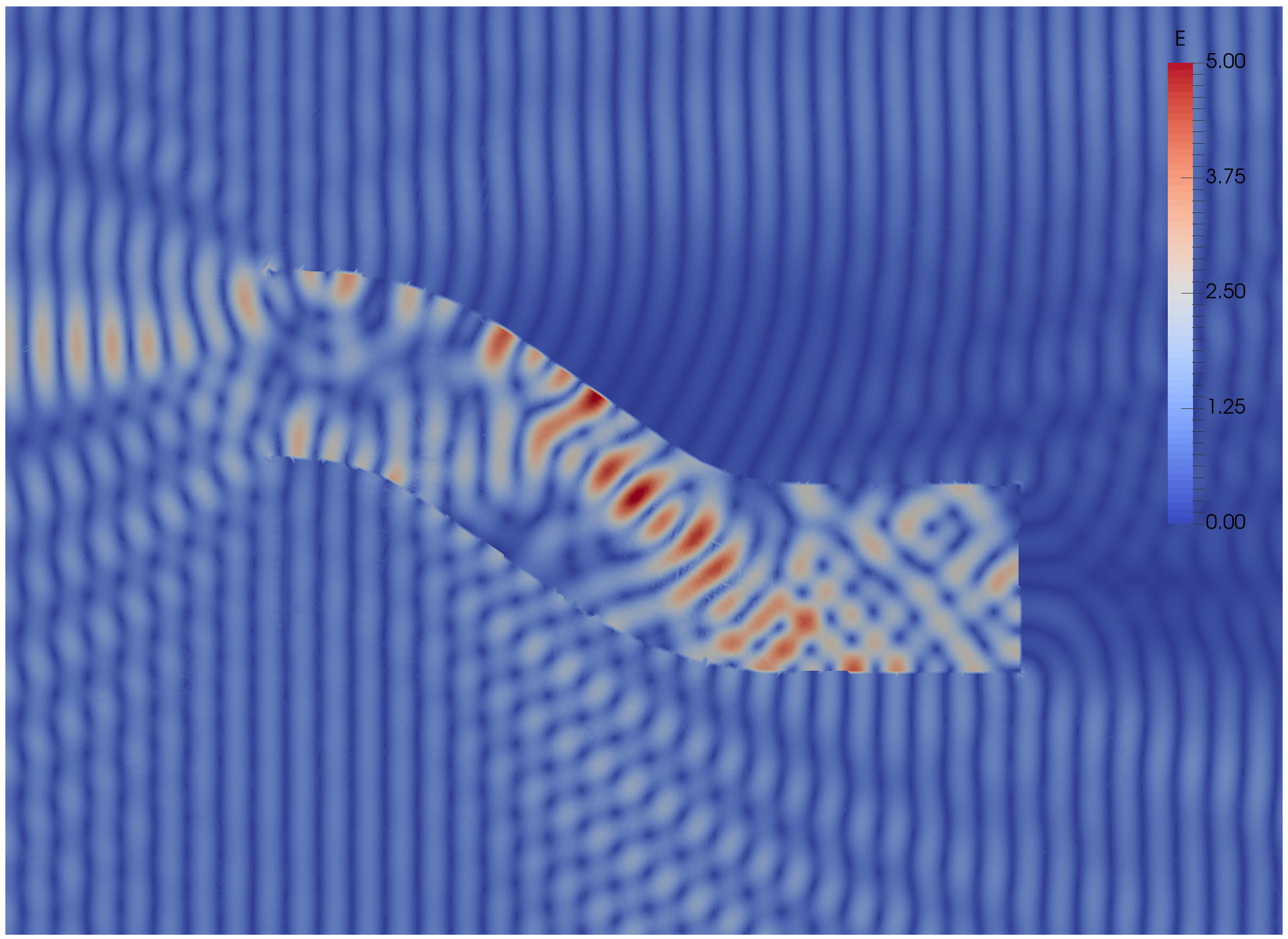
Some results: 2-level DD for Maxwell equations, scattering from the COBRA cavity

f = 10 GHz

f = 16 GHz

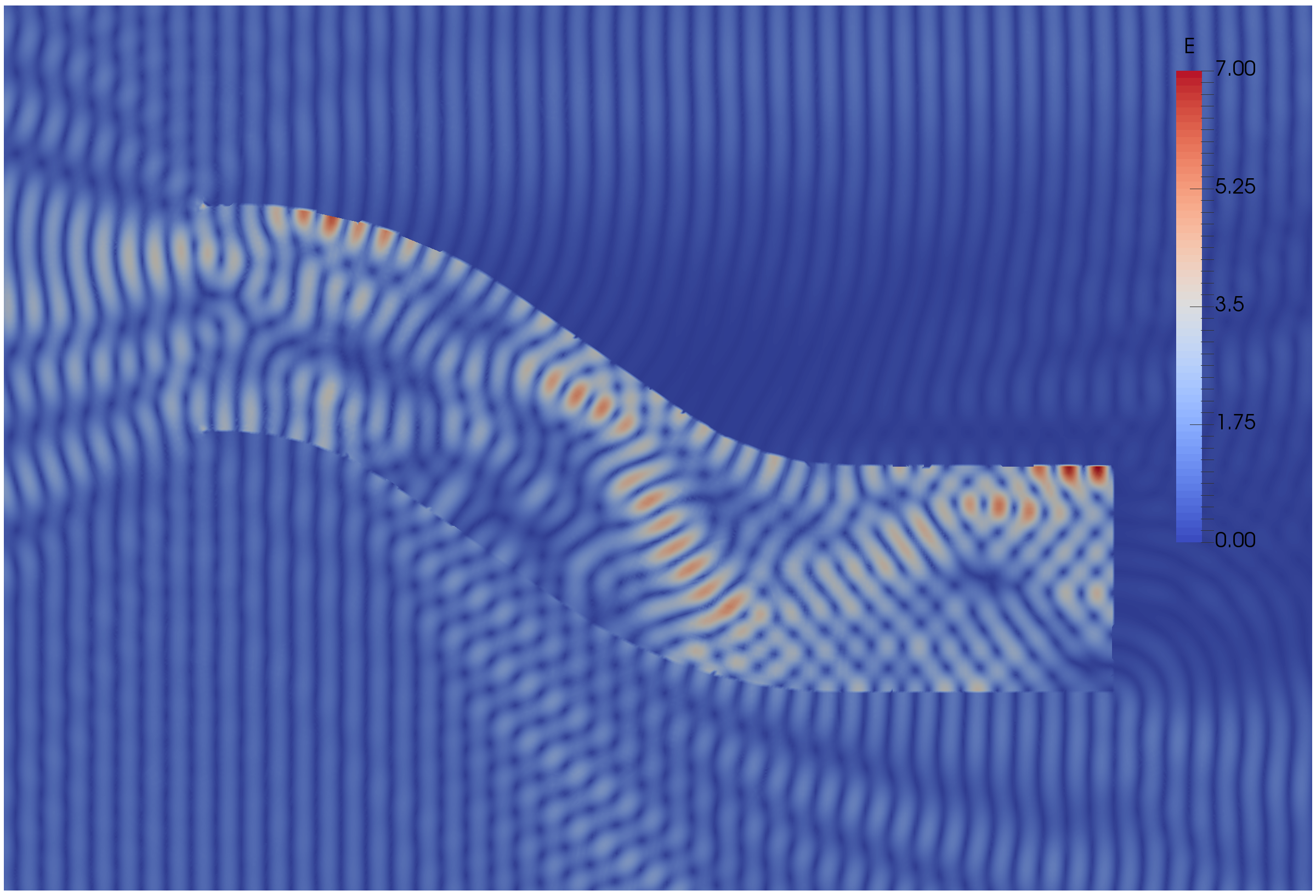
Some results: 2-level DD for Maxwell equations, scattering from the COBRA cavity

order 2 Nedelec edge FE
fine mesh: 10 points per wavelength
coarse mesh: 3.33 points per wavelength
two level ORAS preconditioner with added absorption
f = 10 GHz: $n\approx$ 107 million, $n_c \approx$ 4 million

f = 16 GHz: $n\approx$ 198 million, $n_c \approx$ 7.4 million

$\rightarrow$ coarse problem too large for a direct solver $\Rightarrow$ inexact coarse solve: GMRES + one level ORAS preconditioner

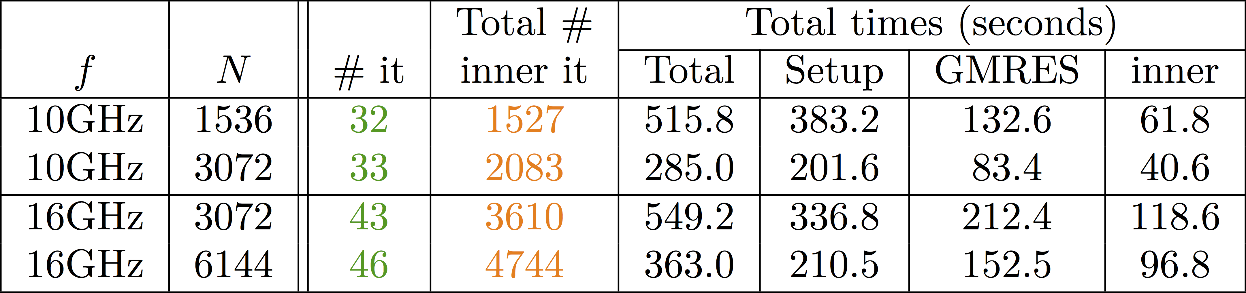
speedup of 1.81 from 1536 to 3072 cores at 10GHz

1.51 from 3072 to 6144 cores at 16GHz

You can find the script here

Here you can use the search bar to search in all FreeFEM examples instead

The list of all matching examples on the right is updated for each new query

Clicking on a search hit or on an example on the right brings up the corresponding script from GitHub

You can also filter the list on the right by selecting one or more intersecting categories on the left tree

Tutorial

What is ffddm ?

Why Domain Decomposition Methods ?

Step 1: Decompose the mesh

Step 2: Define your finite element

Distributed vectors and restriction operators

Partition of unity

Data exchange between neighbors

Step 3: Define your problem

Summary so far: translating your sequential FreeFEM script

Step 1: Decompose the mesh

Solve the linear system

Solve the linear system with the parallel direct solver MUMPS

Step 4: Define the one level DD preconditioner

Step 5: Solve the linear system with preconditioned GMRES

Define a two level DD preconditioner

Build the GenEO coarse space

Build the coarse space from a coarse mesh

Use HPDDM within ffddm

Some results: Heterogeneous 3D elasticity with GenEO

Some results: 2-level DD for Maxwell equations, scattering from the COBRA cavity

Some results: 2-level DD for Maxwell equations, scattering from the COBRA cavity