Optimal Control
Thanks to the function BFGS it is possible to solve complex nonlinear optimization problem within FreeFEM.
For example consider the following inverse problem
where the desired state \(u_d\), the boundary data \(u_\Gamma\) and the observation set \(E\subset\Omega\) are all given. Furthermore let us assume that:
where \(B,C,D\) are separated subsets of \(\Omega\).
To solve this problem by the quasi-Newton BFGS method we need the derivatives of \(J\) with respect to \(b,c,d\). We self explanatory notations, if \(\delta b,\delta c,\delta d\) are variations of \(b,c,d\) we have:
Obviously \(J'_b\) is equal to \(\delta J\) when \(\delta b=1,\delta c=0,\delta d=0\), and so on for \(J'_c\) and \(J'_d\).
All this is implemented in the following program:
 1// Mesh
 2border aa(t=0, 2*pi){x=5*cos(t); y=5*sin(t);};
 3border bb(t=0, 2*pi){x=cos(t); y=sin(t);};
 4border cc(t=0, 2*pi){x=-3+cos(t); y=sin(t);};
 5border dd(t=0, 2*pi){x=cos(t); y =-3+sin(t);};
 6
 7mesh th = buildmesh(aa(70) + bb(35) + cc(35) + dd(35));
 8
 9// Fespace
10fespace Vh(th, P1);
11Vh Ib=((x^2+y^2)<1.0001),
12   Ic=(((x+3)^2+ y^2)<1.0001),
13   Id=((x^2+(y+3)^2)<1.0001),
14   Ie=(((x-1)^2+ y^2)<=4),
15   ud, u, uh, du;
16
17// Problem
18real[int] z(3);
19problem A(u, uh)
20   = int2d(th)(
21        (1+z[0]*Ib+z[1]*Ic+z[2]*Id)*(dx(u)*dx(uh) + dy(u)*dy(uh))
22   )
23   + on(aa, u=x^3-y^3)
24   ;
25
26// Solve
27z[0]=2; z[1]=3; z[2]=4;
28A;
29ud = u;
30
31ofstream f("J.txt");
32func real J(real[int] & Z){
33   for (int i = 0; i < z.n; i++)
34      z[i] =Z[i];
35   A;
36   real s = int2d(th)(Ie*(u-ud)^2);
37   f << s << " ";
38   return s;
39}
40
41// Problem BFGS
42real[int] dz(3), dJdz(3);
43problem B (du, uh)
44   = int2d(th)(
45        (1+z[0]*Ib+z[1]*Ic+z[2]*Id)*(dx(du)*dx(uh) + dy(du)*dy(uh))
46   )
47   + int2d(th)(
48        (dz[0]*Ib+dz[1]*Ic+dz[2]*Id)*(dx(u)*dx(uh) + dy(u)*dy(uh))
49   )
50   +on(aa, du=0)
51   ;
52
53func real[int] DJ(real[int] &Z){
54   for(int i = 0; i < z.n; i++){
55      for(int j = 0; j < dz.n; j++)
56         dz[j] = 0;
57      dz[i] = 1;
58      B;
59      dJdz[i] = 2*int2d(th)(Ie*(u-ud)*du);
60   }
61   return dJdz;
62}
63
64real[int] Z(3);
65for(int j = 0; j < z.n; j++)
66   Z[j]=1;
67
68BFGS(J, DJ, Z, eps=1.e-6, nbiter=15, nbiterline=20);
69cout << "BFGS: J(z) = " << J(Z) << endl;
70for(int j = 0; j < z.n; j++)
71   cout << z[j] << endl;
72
73// Plot
74plot(ud, value=1, ps="u.eps");
In this example the sets \(B,C,D,E\) are circles of boundaries \(bb,cc,dd,ee\) and the domain \(\Omega\) is the circle of boundary \(aa\).
The desired state \(u_d\) is the solution of the PDE for \(b=2,c=3,d=4\). The unknowns are packed into array \(z\).
Note
It is necessary to recopy \(Z\) into \(z\) because one is a local variable while the other one is global.
The program found \(b=2.00125,c=3.00109,d=4.00551\).
Fig. 40 and Fig. 41 show \(u\) at convergence and the successive function evaluations of \(J\).
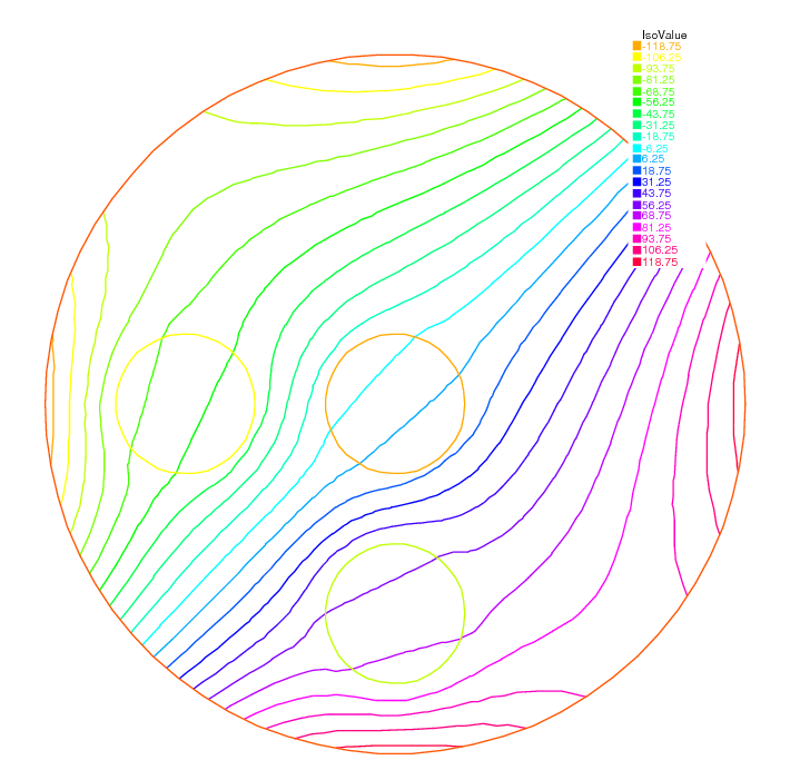
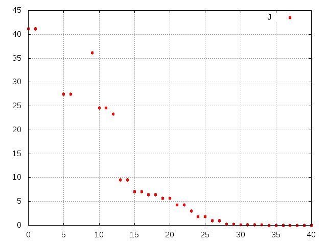
Fig. 41 Successive evaluations of \(J\) by BFGS (5 values above 500 have been removed for readability)
Optimal control
Note that an adjoint state could have been used. Define \(p\) by:
Consequently:
Then the derivatives are found by setting \(\delta b=1, \delta c=\delta d=0\) and so on:
Note
As BFGS stores an \(M\times M\) matrix where \(M\) is the number of unknowns, it is dangerously expensive to use this method when the unknown \(x\) is a Finite Element Function.
One should use another optimizer such as the NonLinear Conjugate Gradient NLCG (also a key word of FreeFEM).