Plotting in Matlab and Octave
Overview
In order to create a plot of a FreeFEM simulation in Matlab© or Octave two steps are necessary:
The mesh, the finite element space connectivity and the simulation data must be exported into files
The files must be imported into the Matlab / Octave workspace. Then the data can be visualized with the ffmatlib library
The steps are explained in more detail below using the example of a stripline capacitor.
Note
Finite element variables must be in P1 or P2. The simulation data can be 2D or 3D.
2D Problem
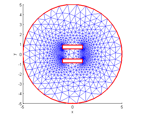
Consider a stripline capacitor problem which is also shown in Fig. 52. On the two boundaries (the electrodes) \(C_{A}\), \(C_{K}\) a Dirichlet condition and on the enclosure \(C_{B}\) a Neumann condition is set. The electrostatic potential \(u\) between the two electrodes is given by the Laplace equation
and the electrostatic field \(\mathbf{E}\) is calculated by
 1int CA=3, CK=4, CB=5;
 2real w2=1.0, h=0.4, d2=0.5;
 3
 4border bottomA(t=-w2,w2){ x=t; y=d2; label=CA;};
 5border rightA(t=d2,d2+h){ x=w2; y=t; label=CA;};
 6border topA(t=w2,-w2){ x=t; y=d2+h; label=CA;};
 7border leftA(t=d2+h,d2){ x=-w2; y=t; label=CA;};
 8
 9border bottomK(t=-w2,w2){ x=t; y=-d2-h; label=CK;};
10border rightK(t=-d2-h,-d2){ x=w2; y=t; label=CK;};
11border topK(t=w2,-w2){ x=t; y=-d2; label=CK;};
12border leftK(t=-d2,-d2-h){ x=-w2; y=t; label=CK;};
13
14border enclosure(t=0,2*pi){x=5*cos(t); y=5*sin(t); label=CB;}
15
16int n=15;
17mesh Th = buildmesh(enclosure(3*n)+
18             bottomA(-w2*n)+topA(-w2*n)+rightA(-h*n)+leftA(-h*n)+
19             bottomK(-w2*n)+topK(-w2*n)+rightK(-h*n)+leftK(-h*n));
20
21fespace Vh(Th,P1);
22
23Vh u,v;
24real u0=2.0;
25
26problem Laplace(u,v,solver=LU) =
27          int2d(Th)(dx(u)*dx(v) + dy(u)*dy(v))
28        + on(CA,u=u0)+on(CK,u=0);
29
30real error=0.01;
31for (int i=0;i<1;i++){
32   Laplace;
33   Th=adaptmesh(Th,u,err=error);
34   error=error/2.0;
35}
36Laplace;
37
38Vh Ex, Ey;
39Ex = -dx(u);
40Ey = -dy(u);
41
42plot(u,[Ex,Ey],wait=true);
Exporting Data
The mesh is stored with the FreeFEM command savemesh(), while the connectivity of the finite element space and the simulation data are stored with the macro commands ffSaveVh() and ffSaveData(). These two commands are located in the ffmatlib.idp file which is included in the ffmatlib. Therefore, to export the stripline capacitor data the following statement sequence must be added to the FreeFEM code:
 1include "ffmatlib.idp"
 2
 3//Save mesh
 4savemesh(Th,"capacitor.msh");
 5//Save finite element space connectivity
 6ffSaveVh(Th,Vh,"capacitor_vh.txt");
 7//Save some scalar data
 8ffSaveData(u,"capacitor_potential.txt");
 9//Save a 2D vector field
10ffSaveData2(Ex,Ey,"capacitor_field.txt");
Importing Data
The mesh file can be loaded into the Matlab / Octave workspace using the ffreadmesh() command. A mesh file consists of three main sections:
The mesh points as nodal coordinates
A list of boundary edges including boundary labels
List of triangles defining the mesh in terms of connectivity
The three data sections mentioned are returned in the variables p, b and t. The finite element space connectivity and the simulation data can be loaded using the ffreaddata() command. Therefore, to load the example data the following statement sequence must be executed in Matlab / Octave:
 1%Add ffmatlib to the search path
 2addpath('add here the link to the ffmatlib');
 3%Load the mesh
 4[p,b,t,nv,nbe,nt,labels]=ffreadmesh('capacitor.msh');
 5%Load the finite element space connectivity
 6vh=ffreaddata('capacitor_vh.txt');
 7%Load scalar data
 8u=ffreaddata('capacitor_potential.txt');
 9%Load 2D vector field data
10[Ex,Ey]=ffreaddata('capacitor_field.txt');
2D Plot Examples
ffpdeplot() is a plot solution for creating patch, contour, quiver, mesh, border, and region plots of 2D geometries. The basic syntax is:
1[handles,varargout] = ffpdeplot(p,b,t,varargin)
varargin specifies parameter name / value pairs to control the plot behaviour.
A table showing all options can be found in the ffmatlib documentation. A small selection of possible plot commands is given as follows:
Plot of the boundary and the mesh:
1ffpdeplot(p,b,t,'Mesh','on','Boundary','on');
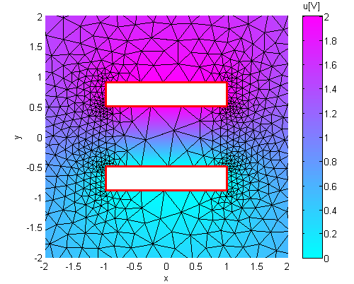
Patch plot (2D map or density plot) including mesh and boundary:
1ffpdeplot(p,b,t,'VhSeq',vh,'XYData',u,'Mesh','on','Boundary','on', ...
2          'XLim',[-2 2],'YLim',[-2 2]);
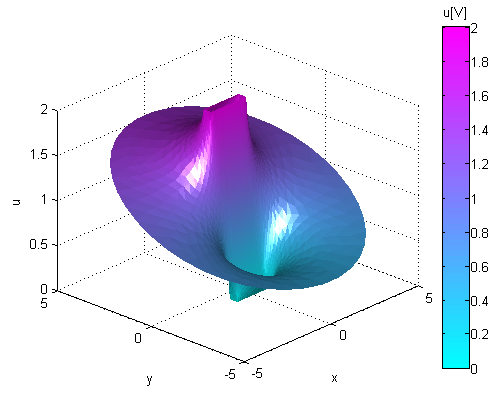
3D surf plot:
1ffpdeplot(p,b,t,'VhSeq',vh,'XYData',u,'ZStyle','continuous', ...
2          'Mesh','off');
3lighting gouraud;
4view([-47,24]);
5camlight('headlight');
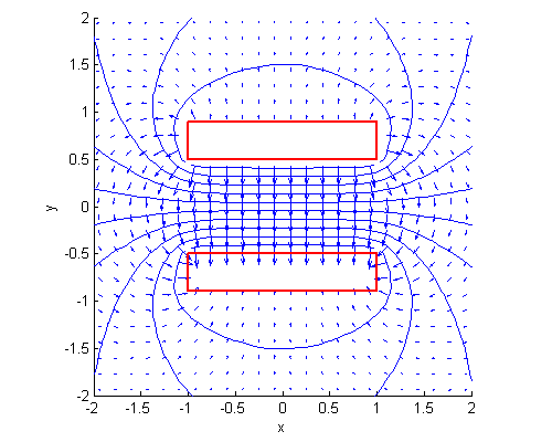
Contour (isovalue) and quiver (vector field) plot:
1ffpdeplot(p,b,t,'VhSeq',vh,'XYData',u,'Mesh','off','Boundary','on', ...
2          'XLim',[-2 2],'YLim',[-2 2],'Contour','on','CColor','b', ...
3          'XYStyle','off', 'CGridParam',[150, 150],'ColorBar','off', ...
4          'FlowData',[Ex,Ey],'FGridParam',[24, 24]);
Download run through example:
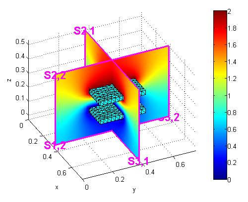
3D Plot Examples
3D problems are handled by the ffpdeplot3D() command, which works similarly to the ffpdeplot() command. In particular in three-dimensions cross sections of the solution can be created. The following example shows a cross-sectional problem of a three-dimensional parallel plate capacitor.
Download run through example: