Eigen value problems

This section depends on your installation of FreeFEM; you need to have compiled ARPACK. This tool is available in FreeFEM if the word eigenvalue appears in line Load:, like:

-- FreeFem++ v*.** (date *** *** ** **:**:** CET ****)
 file : ***.edp
 Load: lg_fem lg_mesh eigenvalue

This tool is based on arpack++, the object-oriented version of ARPACK eigenvalue package [LEHOUCQ1998].

The function EigenValue computes the generalized eigenvalue of \(A u = \lambda B u\). The Shift-invert method is used by default, with sigma =\(\sigma\) the shift of the method.

The matrix \(OP\) is defined with \(A - \sigma B\).

The return value is the number of converged eigenvalues (can be greater than the number of requested eigenvalues nev=)

int k = EigenValue(OP, B, nev=Nev, sigma=Sigma);

where the matrix \(OP= A - \sigma B\) with a solver and boundary condition, and the matrix \(B\).

There is also a functional interface:

int k = EigenValue(n, FOP1, FB, nev=Nev, sigma=Sigma);

where \(n\) is the size of the problem, and the operators are now defined through functions, defining respectively the matrix product of \(OP^{-1}\) and \(B\), as in

int n = OP1.n;
func real[int] FOP1(real[int] & u){ real[int] Au = OP^-1*u; return Au; }
func real[int] FB(real[int] & u){ real[int] Au = B*u; return Au; }

If you want finer control over the method employed in ARPACK, you can specify which mode ARPACK will work with (mode= , see ARPACK documentation [LEHOUCQ1998]). The operators necessary for the chosen mode can be passed through the optional parameters A=, A1=, B=, B1=, (see below).

mode=1: Regular mode for solving \(A u = \lambda u\)
```
1int k = EigenValue(n, A=FOP, mode=1, nev=Nev);
```
where the function FOP defines the matrix product of A
mode=2: Regular inverse mode for solving \(A u = \lambda B u\)
```
1int k = EigenValue(n, A=FOP, B=FB, B1=FB1, mode=2, nev=Nev);
```
where the functions FOP, FB and FB1 define respectively the matrix product of \(A\), \(B\) and \(B^{-1}\)
mode=3: Shift-invert mode for solving \(A u = \lambda B u\)
```
1int k = EigenValue(n, A1=FOP1, B=FB, mode=3, sigma=Sigma, nev=Nev);
```
where the functions FOP1 and FB define respectively the matrix product of \(OP^{-1} = (A - \sigma B)^{-1}\) and \(B\)

You can also specify which subset of eigenvalues you want to compute (which=). The default value is which="LM", for eigenvalues with largest magnitude. "SM" is for smallest magnitude, "LA" for largest algebraic value, "SA" for smallest algebraic value, and "BE" for both ends of the spectrum.

Remark: For complex problems, you need to use the keyword complexEigenValue instead of EigenValue when passing operators through functions.

Note

Boundary condition and Eigenvalue Problems

The locking (Dirichlet) boundary condition is make with exact penalization so we put 1e30=tgv on the diagonal term of the locked degree of freedom (see Finite element chapter). So take Dirichlet boundary condition just on \(A\) and not on \(B\) because we solve \(w=OP^{-1}*B*v\).

If you put locking (Dirichlet) boundary condition on \(B\) matrix (with key work on) you get small spurious modes \((10^{-30})\), due to boundary condition, but if you forget the locking boundary condition on \(B\) matrix (no keywork on) you get huge spurious \((10^{30})\) modes associated to these boundary conditons. We compute only small mode, so we get the good one in this case.

sym= The problem is symmetric (all the eigen value are real)
nev= The number desired eigenvalues (nev) close to the shift.
value= The array to store the real part of the eigenvalues
ivalue= The array to store the imaginary part of the eigenvalues
vector= The FE function array to store the eigenvectors
rawvector= An array of type real[int,int] to store eigenvectors by column.

For real non symmetric problems, complex eigenvectors are given as two consecutive vectors, so if eigenvalue \(k\) and \(k+1\) are complex conjugate eigenvalues, the \(k\)th vector will contain the real part and the \(k+1\)th vector the imaginary part of the corresponding complex conjugate eigenvectors.
tol= The relative accuracy to which eigenvalues are to be determined;
sigma= The shift value;
maxit= The maximum number of iterations allowed;
ncv= The number of Arnoldi vectors generated at each iteration of ARPACK;
mode= The computational mode used by ARPACK (see above);
which= The requested subset of eigenvalues (see above).

Tip

Laplace eigenvalue

In the first example, we compute the eigenvalues and the eigenvectors of the Dirichlet problem on square \(\Omega=]0,\pi[^2\).

The problem is to find: \(\lambda\), and \(\nabla u_{\lambda}\) in \(\mathbb{R}{\times} H^1_0(\Omega)\)

\[\int_\Omega \nabla u_{\lambda} \nabla v = \lambda \int_\Omega u v \quad \forall v \in H^1_0(\Omega)\]

The exact eigenvalues are \(\lambda_{n,m} =(n^2+m^2), (n,m)\in {\mathbb{N}_*}^2\) with the associated eigenvectors are \(u_{{m,n}}=\sin(nx)*\sin(my)\).

We use the generalized inverse shift mode of the arpack++ library, to find 20 eigenvalues and eigenvectors close to the shift value \(\sigma=20\).

// Parameters
verbosity=0;
real sigma = 20; //value of the shift
int nev = 20; //number of computed eigen value close to sigma

// Mesh
mesh Th = square(20, 20, [pi*x, pi*y]);

// Fespace
fespace Vh(Th, P2);
Vh u1, u2;

// Problem
// OP = A - sigma B ; // the shifted matrix
varf op (u1, u2)
    = int2d(Th)(
          dx(u1)*dx(u2)
        + dy(u1)*dy(u2)
        - sigma* u1*u2
    )
    + on(1, 2, 3, 4, u1=0)
    ;

varf b ([u1], [u2]) = int2d(Th)(u1*u2); //no boundary condition

matrix OP = op(Vh, Vh, solver=Crout, factorize=1); //crout solver because the matrix in not positive
matrix B = b(Vh, Vh, solver=CG, eps=1e-20);

// important remark:
// the boundary condition is make with exact penalization:
// we put 1e30=tgv on the diagonal term of the lock degree of freedom.
// So take Dirichlet boundary condition just on $a$ variational form
// and not on $b$ variational form.
// because we solve $ w=OP^-1*B*v $

// Solve
real[int] ev(nev); //to store the nev eigenvalue
Vh[int] eV(nev); //to store the nev eigenvector

int k = EigenValue(OP, B, sym=true, sigma=sigma, value=ev, vector=eV,
    tol=1e-10, maxit=0, ncv=0);

// Display & Plot
for (int i = 0; i < k; i++){
    u1 = eV[i];
    real gg = int2d(Th)(dx(u1)*dx(u1) + dy(u1)*dy(u1));
    real mm = int2d(Th)(u1*u1) ;
    cout << "lambda[" << i << "] = " << ev[i] << ", err= " << int2d(Th)(dx(u1)*dx(u1) + dy(u1)*dy(u1) - (ev[i])*u1*u1) << endl;
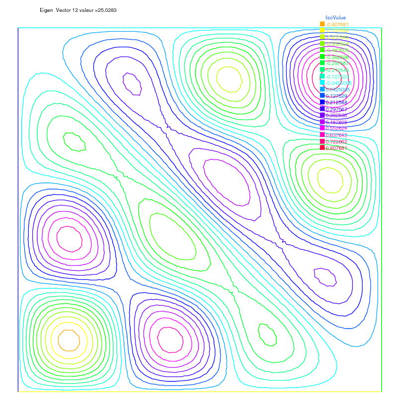
    plot(eV[i], cmm="Eigen Vector "+i+" value ="+ev[i], wait=true, value=true);
}

The output of this example is:

lambda[0] = 5.0002, err= -1.46519e-11
lambda[1] = 8.00074, err= -4.05158e-11
lambda[2] = 10.0011, err= 2.84925e-12
lambda[3] = 10.0011, err= -7.25456e-12
lambda[4] = 13.002, err= -1.74257e-10
lambda[5] = 13.0039, err= 1.22554e-11
lambda[6] = 17.0046, err= -1.06274e-11
lambda[7] = 17.0048, err= 1.03883e-10
lambda[8] = 18.0083, err= -4.05497e-11
lambda[9] = 20.0096, err= -2.21678e-13
lambda[10] = 20.0096, err= -4.16212e-14
lambda[11] = 25.014, err= -7.42931e-10
lambda[12] = 25.0283, err= 6.77444e-10
lambda[13] = 26.0159, err= 3.19864e-11
lambda[14] = 26.0159, err= -4.9652e-12
lambda[15] = 29.0258, err= -9.99573e-11
lambda[16] = 29.0273, err= 1.38242e-10
lambda[17] = 32.0449, err= 1.2522e-10
lambda[18] = 34.049, err= 3.40213e-11
lambda[19] = 34.0492, err= 2.41751e-10

EigenValueProblems1 — Fig. 159 Isovalue of 11th eigenvector \(u_{4,3}-u_{3,4}\)

EigenValueProblems2 — Fig. 160 Isovalue of 12th eigenvector \(u_{4,3}+u_{3,4}\)

Here you can use the search bar to search in all FreeFEM examples instead

The list of all matching examples on the right is updated for each new query

Clicking on a search hit or on an example on the right brings up the corresponding script from GitHub

You can also filter the list on the right by selecting one or more intersecting categories on the left tree

Eigen value problems