Newton Method for the Steady Navier-Stokes equations
The problem is find the velocity field \(\mathbf{u}=(u_i)_{i=1}^d\) and the pressure \(p\) of a Flow satisfying in the domain \(\Omega \subset \mathbb{R}^d (d=2,3)\):
where \(\nu\) is the viscosity of the fluid, \(\nabla = (\partial_i )_{i=1}^d\), the dot product is \(\cdot\), and \(\Delta = \nabla\cdot\nabla\) with the same boundary conditions (\(\mathbf{u}\) is given on \(\Gamma\)).
The weak form is find \(\mathbf{u}, p\) such that for \(\forall \mathbf{v}\) (zero on \(\Gamma\)), and \(\forall q\):
The Newton Algorithm to solve nonlinear problem is:
Find \(u\in V\) such that \(F(u)=0\) where \(F : V \mapsto V\).
choose \(u_0\in \mathbb{R}^n\) , ;
for ( \(i =0\); \(i\) < niter; \(i = i+1\))
solve \(DF(u_i) w_i = F(u_i)\);
\(u_{i+1} = u_i - w_i\);
break \(|| w_i|| < \varepsilon\).
Where \(DF(u)\) is the differential of \(F\) at point \(u\), this is a linear application such that:
For Navier Stokes, \(F\) and \(DF\) are:
So the Newton algorithm become:
1// Parameters
2real R = 5.;
3real L = 15.;
4
5real nu = 1./50.;
6real nufinal = 1/200.;
7real cnu = 0.5;
8
9real eps = 1e-6;
10
11verbosity = 0;
12
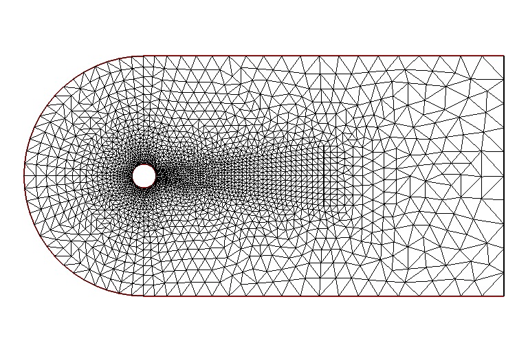
13// Mesh
14border cc(t=0, 2*pi){x=cos(t)/2.; y=sin(t)/2.; label=1;}
15border ce(t=pi/2, 3*pi/2){x=cos(t)*R; y=sin(t)*R; label=1;}
16border beb(tt=0, 1){real t=tt^1.2; x=t*L; y=-R; label=1;}
17border beu(tt=1, 0){real t=tt^1.2; x=t*L; y=R; label=1;}
18border beo(t=-R, R){x=L; y=t; label=0;}
19border bei(t=-R/4, R/4){x=L/2; y=t; label=0;}
20mesh Th = buildmesh(cc(-50) + ce(30) + beb(20) + beu(20) + beo(10) + bei(10));
21plot(Th);
22
23//bounding box for the plot
24func bb = [[-1,-2],[4,2]];
25
26// Fespace
27fespace Xh(Th, P2);
28Xh u1, u2;
29Xh v1,v2;
30Xh du1,du2;
31Xh u1p,u2p;
32
33fespace Mh(Th,P1);
34Mh p;
35Mh q;
36Mh dp;
37Mh pp;
38
39// Macro
40macro Grad(u1,u2) [dx(u1), dy(u1), dx(u2),dy(u2)] //
41macro UgradV(u1,u2,v1,v2) [[u1,u2]'*[dx(v1),dy(v1)],
42 [u1,u2]'*[dx(v2),dy(v2)]] //
43macro div(u1,u2) (dx(u1) + dy(u2)) //
44
45// Initialization
46u1 = (x^2+y^2) > 2;
47u2 = 0;
48
49// Viscosity loop
50while(1){
51 int n;
52 real err=0;
53 // Newton loop
54 for (n = 0; n < 15; n++){
55 // Newton
56 solve Oseen ([du1, du2, dp], [v1, v2, q])
57 = int2d(Th)(
58 nu * (Grad(du1,du2)' * Grad(v1,v2))
59 + UgradV(du1,du2, u1, u2)' * [v1,v2]
60 + UgradV( u1, u2,du1,du2)' * [v1,v2]
61 - div(du1,du2) * q
62 - div(v1,v2) * dp
63 - 1e-8*dp*q //stabilization term
64 )
65 - int2d(Th) (
66 nu * (Grad(u1,u2)' * Grad(v1,v2))
67 + UgradV(u1,u2, u1, u2)' * [v1,v2]
68 - div(u1,u2) * q
69 - div(v1,v2) * p
70 )
71 + on(1, du1=0, du2=0)
72 ;
73
74 u1[] -= du1[];
75 u2[] -= du2[];
76 p[] -= dp[];
77
78 real Lu1=u1[].linfty, Lu2=u2[].linfty, Lp=p[].linfty;
79 err = du1[].linfty/Lu1 + du2[].linfty/Lu2 + dp[].linfty/Lp;
80
81 cout << n << " err = " << err << " " << eps << " rey = " << 1./nu << endl;
82 if(err < eps) break; //converge
83 if( n>3 && err > 10.) break; //blowup
84 }
85
86 if(err < eps){ //converge: decrease $\nu$ (more difficult)
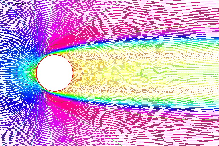
87 // Plot
88 plot([u1, u2], p, wait=1, cmm=" rey = " + 1./nu , coef=0.3, bb=bb);
89
90 // Change nu
91 if( nu == nufinal) break;
92 if( n < 4) cnu = cnu^1.5; //fast converge => change faster
93 nu = max(nufinal, nu* cnu); //new viscosity
94
95 // Update
96 u1p = u1;
97 u2p = u2;
98 pp = p;
99 }
100 else{ //blowup: increase $\nu$ (more simple)
101 assert(cnu< 0.95); //the method finally blowup
102
103 // Recover nu
104 nu = nu/cnu;
105 cnu= cnu^(1./1.5); //no conv. => change lower
106 nu = nu* cnu; //new viscosity
107 cout << " restart nu = " << nu << " Rey = " << 1./nu << " (cnu = " << cnu << " ) \n";
108
109 // Recover a correct solution
110 u1 = u1p;
111 u2 = u2p;
112 p = pp;
113 }
114}
Note
We use a trick to make continuation on the viscosity \(\nu\), because the Newton method blowup owe start with the final viscosity \(\nu\).
\(\nu\) is gradually increased to the desired value.