Algorithms & Optimization
Conjugate Gradient/GMRES
Suppose we want to solve the Euler problem (here \(x\) has nothing to do with the reserved variable for the first coordinate in FreeFEM):
find \(x\in \mathbb{R}^n\) such that
where \(J\) is a function (to minimize for example) from \(\mathbb{R}^n\) to \(\mathbb{R}\).
If the function is convex we can use the conjugate gradient algorithm to solve the problem, and we just need the function (named dJ for example) which computes \(\nabla J\), so the parameters are the name of that function with prototype func real[int] dJ(real[int] &xx); which computes \(\nabla J\), and a vector x of type (of course the number 20 can be changed) real[int] x(20); to initialize the process and get the result.
Given an initial value \(\mathbf{x}^{(0)}\), a maximum number \(i_{\max}\) of iterations, and an error tolerance \(0<\epsilon<1\):
Put \(\mathbf{x}=\mathbf{x}^{(0)}\) and write
1NLCG(dJ, x, precon=M, nbiter=imax, eps=epsilon, stop=stopfunc);
will give the solution of \(\mathbf{x}\) of \(\nabla J(\mathbf{x})=0\).
We can omit parameters precon, nbiter, eps, stop.
Here \(M\) is the preconditioner whose default is the identity matrix.
The stopping test is
Writing the minus value in eps=, i.e.,
1NLCG(dJ, x, precon=M, nbiter=imax, eps=-epsilon);
We can use the stopping test:
The parameters of these three functions are:
nbiter=set the number of iteration (by default 100)precon=set the preconditioner function (Pfor example) by default it is the identity, note the prototype isfunc real[int] P(real[int] &x).eps=set the value of the stop test \(\varepsilon\) (\(=10^{-6}\) by default) if positive then relative test \(||\nabla J(x)||_P\leq \varepsilon||\nabla J(x_0)||_P\), otherwise the absolute test is \(||\nabla J(x)||_P^2\leq |\varepsilon|\).veps=set and return the value of the stop test, if positive, then relative test is \(||\nabla J(x)||_P\leq \varepsilon||\nabla J(x_0)||_P\), otherwise the absolute test is \(||\nabla J(x)||_P^2\leq |\varepsilon|\). The return value is minus the real stop test (remark: it is useful in loop).stop=stopfuncadd your test function to stop before theepscriterion. The prototype for the functionstopfuncis1func bool stopfunc(int iter, real[int] u, real[int] g)
where
uis the current solution, andg, the current gradient, is not preconditioned.
Tip
For a given function \(b\), let us find the minimizer \(u\) of the function
under the boundary condition \(u=0\) on \(\partial\Omega\).
 1fespace Ph(Th, P0);
 2Ph alpha; //store df(|nabla u|^2)
 3
 4// The function J
 5//J(u) = 1/2 int_Omega f(|nabla u|^2) - int_Omega u b
 6func real J (real[int] & u){
 7   Vh w;
 8   w[] = u;
 9   real r = int2d(Th)(0.5*f(dx(w)*dx(w) + dy(w)*dy(w)) - b*w);
10   cout << "J(u) = " << r << " " << u.min << " " << u.max << endl;
11   return r;
12}
13
14// The gradient of J
15func real[int] dJ (real[int] & u){
16   Vh w;
17   w[] = u;
18   alpha = df(dx(w)*dx(w) + dy(w)*dy(w));
19   varf au (uh, vh)
20      = int2d(Th)(
21           alpha*(dx(w)*dx(vh) + dy(w)*dy(vh))
22         - b*vh
23      )
24      + on(1, 2, 3, 4, uh=0)
25      ;
26
27   u = au(0, Vh);
28   return u; //warning: no return of local array
29}
We also want to construct a preconditioner \(C\) with solving the problem:
find \(u_h \in V_{0h}\) such that:
where \(\alpha=f'(|\nabla u|^2)\).
 1alpha = df(dx(u)*dx(u) + dy(u)*dy(u));
 2varf alap (uh, vh)
 3   = int2d(Th)(
 4        alpha*(dx(uh)*dx(vh) + dy(uh)*dy(vh))
 5   )
 6   + on(1, 2, 3, 4, uh=0)
 7   ;
 8
 9varf amass(uh, vh)
10   = int2d(Th)(
11        uh*vh
12   )
13   + on(1, 2, 3, 4, uh=0)
14   ;
15
16matrix Amass = amass(Vh, Vh, solver=CG);
17matrix Alap= alap(Vh, Vh, solver=Cholesky, factorize=1);
18
19// Preconditionner
20func real[int] C(real[int] & u){
21   real[int] w = u;
22   u = Alap^-1*w;
23   return u; //warning: no return of local array variable
24}
To solve the problem, we make 10 iterations of the conjugate gradient, recompute the preconditioner and restart the conjugate gradient:
 1int conv=0;
 2for(int i = 0; i < 20; i++){
 3   conv = NLCG(dJ, u[], nbiter=10, precon=C, veps=eps, verbosity=5);
 4   if (conv) break;
 5
 6   alpha = df(dx(u)*dx(u) + dy(u)*dy(u));
 7   Alap = alap(Vh, Vh, solver=Cholesky, factorize=1);
 8   cout << "Restart with new preconditionner " << conv << ", eps =" << eps << endl;
 9}
10
11// Plot
12plot (u, wait=true, cmm="solution with NLCG");
For a given symmetric positive matrix \(A\), consider the quadratic form
then \(J(\mathbf{x})\) is minimized by the solution \(\mathbf{x}\) of \(A\mathbf{x}=\mathbf{b}\).
In this case, we can use the function AffineCG
1AffineCG(A, x, precon=M, nbiter=imax, eps=epsilon, stop=stp);
If \(A\) is not symmetric, we can use GMRES(Generalized Minimum Residual) algorithm by
1AffineGMRES(A, x, precon=M, nbiter=imax, eps=epsilon);
Also, we can use the non-linear version of GMRES algorithm (the function \(J\) is just convex)
1AffineGMRES(dJ, x, precon=M, nbiter=imax, eps=epsilon);
For the details of these algorithms, refer to [PIRONNEAU1998], Chapter IV, 1.3.
Algorithms for Unconstrained Optimization
Two algorithms of COOOL package are interfaced with the Newton Raphson method (called Newton) and the BFGS method.
These two are directly available in FreeFEM (no dynamical link to load).
Be careful with these algorithms, because their implementation uses full matrices.
We also provide several optimization algorithms from the NLopt library as well as an interface for Hansen’s implementation of CMAES (a MPI version of this one is also available).
Example of usage for BFGS or CMAES
Tip
BFGS
 1real[int] b(10), u(10);
 2
 3//J
 4func real J (real[int] & u){
 5   real s = 0;
 6   for (int i = 0; i < u.n; i++)
 7      s += (i+1)*u[i]*u[i]*0.5 - b[i]*u[i];
 8   if (debugJ)
 9      cout << "J = " << s << ", u = " << u[0] << " " << u[1] << endl;
10   return s;
11}
12
13//the gradient of J (this is a affine version (the RHS is in)
14func real[int] DJ (real[int] &u){
15   for (int i = 0; i < u.n; i++)
16      u[i] = (i+1)*u[i];
17   if (debugdJ)
18      cout << "dJ: u = " << u[0] << " " << u[1] << " " << u[2] << endl;
19   u -= b;
20   if (debugdJ)
21      cout << "dJ-b: u = " << u[0] << " " << u[1] << " " << u[2] << endl;
22   return u; //return of global variable ok
23}
24
25b=1;
26u=2;
27BFGS(J, DJ, u, eps=1.e-6, nbiter=20, nbiterline=20);
28cout << "BFGS: J(u) = " << J(u) << ", err = " << error(u, b) << endl;
It is almost the same a using the CMA evolution strategy except, that since it is a derivative free optimizer, the dJ argument is omitted and there are some other named parameters to control the behavior of the algorithm.
With the same objective function as above, an example of utilization would be (see CMAES Variational inequality for a complete example):
1load "ff-cmaes"
2//define J, u, ...
3real min = cmaes(J, u, stopTolFun=1e-6, stopMaxIter=3000);
4cout << "minimum value is " << min << " for u = " << u << endl;
This algorithm works with a normal multivariate distribution in the parameters space and tries to adapt its covariance matrix using the information provided by the successive function evaluations (see NLopt documentation for more details). Therefore, some specific parameters can be passed to control the starting distribution, size of the sample generations, etc… Named parameters for this are the following:
seed=Seed for random number generator (valis an integer). No specified value will lead to a clock based seed initialization.initialStdDev=Value for the standard deviations of the initial covariance matrix (valis a real). If the value \(\sigma\) is passed, the initial covariance matrix will be set to \(\sigma I\). The expected initial distance between initial \(X\) and the \(argmin\) should be roughly initialStdDev. Default is 0.3.initialStdDevs=Same as above except that the argument is an array allowing to set a value of the initial standard deviation for each parameter. Entries differing by several orders of magnitude should be avoided (if it can’t be, try rescaling the problem).stopTolFun=Stops the algorithm if function value differences are smaller than the passed one, default is \(10^{-12}\).stopTolFunHist=Stops the algorithm if function value differences from the best values are smaller than the passed one, default is 0 (unused).stopTolX=Stopping criteria is triggered if step sizes in the parameters space are smaller than this real value, default is 0.stopTolXFactor=Stopping criteria is triggered when the standard deviation increases more than this value. The default value is \(10^{3}\).stopMaxFunEval=Stops the algorithm whenstopMaxFunEvalfunction evaluations have been done. Set to \(900(n+3)^{2}\) by default, where \(n\) is the parameters space dimension.stopMaxIter=Integer stopping the search whenstopMaxItergenerations have been sampled. Unused by default.popsize=Integer value used to change the sample size. The default value is \(4+ \lfloor 3\ln (n) \rfloor\). Increasing the population size usually improves the global search capabilities at the cost of, at most, a linear reduction of the convergence speed with respect topopsize.paramFile=Thisstringtype parameter allows the user to pass all the parameters using an extern file, as in Hansen’s original code. More parameters related to the CMA-ES algorithm can be changed with this file. Note that the parameters passed to the CMAES function in the FreeFEM script will be ignored if an input parameters file is given.
IPOPT
The ff-Ipopt package is an interface for the IPOPT [WÄCHTER2006] optimizer.
IPOPT is a software library for large scale, non-linear, constrained optimization.
It implements a primal-dual interior point method along with filter method based line searches.
IPOPT needs a direct sparse symmetric linear solver.
If your version of FreeFEM has been compiled with the --enable-downlad tag, it will automatically be linked with a sequential version of MUMPS.
An alternative to MUMPS would be to download the HSL subroutines (see Compiling and Installing the Java Interface JIPOPT) and place them in the /ipopt/Ipopt-3.10.2/ThirdParty/HSL directory of the FreeFEM downloads folder before compiling.
Short description of the algorithm
In this section, we give a very brief glimpse at the underlying mathematics of IPOPT. For a deeper introduction on interior methods for nonlinear smooth optimization, one may consult [FORSGREN2002], or [WÄCHTER2006] for more IPOPT specific elements. IPOPT is designed to perform optimization for both equality and inequality constrained problems. However, nonlinear inequalities are rearranged before the beginning of the optimization process in order to restrict the panel of nonlinear constraints to those of the equality kind. Each nonlinear inequality is transformed into a pair of simple bound inequalities and nonlinear equality constraints by the introduction of as many slack variables as is needed : \(c_{i}(x)\leq 0\) becomes \(c_{i}(x) + s_{i} = 0\) and \(s_{i}\leq 0\), where \(s_{i}\) is added to the initial variables of the problems \(x_{i}\). Thus, for convenience, we will assume that the minimization problem does not contain any nonlinear inequality constraint. It means that, given a function \(f:\mathbb{R}^{n}\mapsto\mathbb{R}\), we want to find:
Where \(c:\mathbb{R}^{n}\rightarrow\mathbb{R}^{m}\) and \(x_{l},x_{u}\in\mathbb{R}^{n}\) and inequalities hold componentwise. The \(f\) function as well as the constraints \(c\) should be twice-continuously differentiable.
As a barrier method, interior points algorithms try to find a Karush-Kuhn-Tucker point for (25) by solving a sequence of problems, unconstrained with respect to the inequality constraints, of the form:
Where \(\mu\) is a positive real number and
The remaining equality constraints are handled with the usual Lagrange multipliers method. If the sequence of barrier parameters \(\mu\) converge to 0, intuition suggests that the sequence of minimizers of (26) converge to a local constrained minimizer of (25). For a given \(\mu\), (26) is solved by finding \((x_{\mu},\lambda_{\mu})\in\mathbb{R}^{n}\times\mathbb{R}^{m}\) such that:
The derivations for \(\nabla B\) only holds for the \(x\) variables, so that:
If we respectively call \(z_{u}(x,\mu) = \left(\mu/(x_{u,1}-x_{1}),\dots, \mu/(x_{u,n}-x_{n})\right)\) and \(z_{l}(x,\mu)\) the other vector appearing in the above equation, then the optimum \((x_{\mu},\lambda_{\mu})\) satisfies:
In this equation, the \(z_l\) and \(z_u\) vectors seem to play the role of Lagrange multipliers for the simple bound inequalities, and indeed, when \(\mu\rightarrow 0\), they converge toward some suitable Lagrange multipliers for the KKT conditions, provided some technical assumptions are fulfilled (see [FORSGREN2002]).
Equation (28) is solved by performing a Newton method in order to find a solution of (27) for each of the decreasing values of \(\mu\). Some order 2 conditions are also taken into account to avoid convergence to local maximizers, see [FORSGREN2002] for details about them. In the most classic IP algorithms, the Newton method is directly applied to (27). This is in most case inefficient due to frequent computation of infeasible points. These difficulties are avoided in Primal-Dual interior point methods where (27) is transformed into an extended system where \(z_u\) and \(z_l\) are treated as unknowns and the barrier problems are finding \((x,\lambda,z_u,z_l)\in\mathbb{R}^n\times\mathbb{R}^m\times\mathbb{R}^n\times\mathbb{R}^n\) such that:
Where if \(a\) is a vector of \(\mathbb{R}^n\), \(A\) denotes the diagonal matrix \(A=(a_i \delta_{ij})_{1\leq i,j\leq n}\) and \(e\in\mathbb{R}^{n} = (1,1,\dots,1)\). Solving this nonlinear system by the Newton method is known as being the primal-dual interior point method. Here again, more details are available in [FORSGREN2002]. Most actual implementations introduce features in order to globalize the convergence capability of the method, essentially by adding some line-search steps to the Newton algorithm, or by using trust regions. For the purpose of IPOPT, this is achieved by a filter line search methods, the details of which can be found in [WÄCHTER2006].
More IPOPT specific features or implementation details can be found in [WÄCHTER2006]. We will just retain that IPOPT is a smart Newton method for solving constrained optimization problems, with global convergence capabilities due to a robust line search method (in the sense that the algorithm will converge no matter the initializer). Due to the underlying Newton method, the optimization process requires expressions of all derivatives up to the order 2 of the fitness function as well as those of the constraints. For problems whose Hessian matrices are difficult to compute or lead to high dimensional dense matrices, it is possible to use a BFGS approximation of these objects at the cost of a much slower convergence rate.
IPOPT in FreeFEM
Calling the IPOPT optimizer in a FreeFEM script is done with the IPOPT function included in the ff-Ipopt dynamic library.
IPOPT is designed to solve constrained minimization problems in the form:
Where \(\mathrm{ub}\) and \(\mathrm{lb}\) stand for “upper bound” and “lower bound”. If for some \(i, 1\leq i\leq m\) we have \(c_{i}^{\mathrm{lb}} = c_{i}^{\mathrm{ub}}\), it means that \(c_{i}\) is an equality constraint, and an inequality one if \(c_{i}^{\mathrm{lb}} < c_{i}^{\mathrm{ub}}\).
There are different ways to pass the fitness function and constraints.
The more general one is to define the functions using the keyword func.
Any returned matrix must be a sparse one (type matrix, not a real[int,int]):
1func real J (real[int] &X) {...} //Fitness Function, returns a scalar
2func real[int] gradJ (real[int] &X) {...} //Gradient is a vector
3
4func real[int] C (real[int] &X) {...} //Constraints
5func matrix jacC (real[int] &X) {...} //Constraints Jacobian
Warning
In the current version of FreeFEM, returning a matrix object that is local to a function block leads to undefined results.
For each sparse matrix returning function you define, an extern matrix object has to be declared, whose associated function will overwrite and return on each call.
Here is an example for jacC:
1matrix jacCBuffer; //just declare, no need to define yet
2func matrix jacC (real[int] &X){
3   ...//fill jacCBuffer
4   return jacCBuffer;
5}
Warning
IPOPT requires the structure of each matrix at the initialization of the algorithm.
Some errors may occur if the matrices are not constant and are built with the matrix A = [I,J,C] syntax, or with an intermediary full matrix (real[int,int]), because any null coefficient is discarded during the construction of the sparse matrix.
It is also the case when making matrices linear combinations, for which any zero coefficient will result in the suppression of the matrix from the combination.
Some controls are available to avoid such problems.
Check the named parameter descriptions (checkindex, structhess and structjac can help).
We strongly advice to use varf as much as possible for the matrix forging.
The Hessian returning function is somewhat different because it has to be the Hessian of the Lagrangian function:
Your Hessian function should then have the following prototype:
1matrix hessianLBuffer; //Just to keep it in mind
2func matrix hessianL (real[int] &X, real sigma, real[int] &lambda){...}
If the constraints functions are all affine, or if there are only simple bound constraints, or no constraint at all, the Lagrangian Hessian is equal to the fitness function Hessian, one can then omit the sigma and lambda parameters:
1matrix hessianJBuffer;
2func matrix hessianJ (real[int] &X){...} //Hessian prototype when constraints are affine
When these functions are defined, IPOPT is called this way:
1real[int] Xi = ... ; //starting point
2IPOPT(J, gradJ, hessianL, C, jacC, Xi, /*some named parameters*/);
If the Hessian is omitted, the interface will tell IPOPT to use the (L)BFGS approximation (it can also be enabled with a named parameter, see further). Simple bound or unconstrained problems do not require the constraints part, so the following expressions are valid:
1IPOPT(J, gradJ, C, jacC, Xi, ... ); //IPOPT with BFGS
2IPOPT(J, gradJ, hessianJ, Xi, ... ); //Newton IPOPT without constraints
3IPOPT(J, gradJ, Xi, ... ); //BFGS, no constraints
Simple bounds are passed using the lb and ub named parameters, while constraint bounds are passed with the clb and cub ones.
Unboundedness in some directions can be achieved by using the \(1e^{19}\) and \(-1e^{19}\) values that IPOPT recognizes as \(+\infty\) and \(-\infty\):
1real[int] xlb(n), xub(n), clb(m), cub(m);
2//fill the arrays...
3IPOPT(J, gradJ, hessianL, C, jacC, Xi, lb=xlb, ub=xub, clb=clb, cub=cub, /*some other named parameters*/);
P2 fitness function and affine constraints function : In the case where the fitness function or constraints function can be expressed respectively in the following forms:
where \(A\) and \(b\) are constant, it is possible to directly pass the \((A,b)\) pair instead of defining 3 (or 2) functions. It also indicates to IPOPT that some objects are constant and that they have to be evaluated only once, thus avoiding multiple copies of the same matrix. The syntax is:
1// Affine constraints with "standard" fitness function
2matrix A = ... ; //linear part of the constraints
3real[int] b = ... ; //constant part of constraints
4IPOPT(J, gradJ, hessianJ, [A, b], Xi, /*bounds and named parameters*/);
5//[b, A] would work as well.
Note that if you define the constraints in this way, they don’t contribute to the Hessian, so the Hessian should only take one real[int] as an argument.
1// Affine constraints and P2 fitness func
2matrix A = ... ; //bilinear form matrix
3real[int] b = ... ; //linear contribution to f
4matrix Ac = ... ; //linear part of the constraints
5real[int] bc = ... ; //constant part of constraints
6IPOPT([A, b], [Ac, bc], Xi, /*bounds and named parameters*/);
If both objective and constraint functions are given this way, it automatically activates the IPOPT mehrotra_algorithm option (better for linear and quadratic programming according to the documentation).
Otherwise, this option can only be set through the option file (see the named parameters section).
A false case is the one of defining \(f\) in this manner while using standard functions for the constraints:
1matrix A = ... ; //bilinear form matrix
2real[int] b = ... ; //linear contribution to f
3func real[int] C(real[int] &X){...} //constraints
4func matrix jacC(real[int] &X){...} //constraints Jacobian
5IPOPT([A, b], C, jacC, Xi, /*bounds and named parameters*/);
Indeed, when passing [A, b] in order to define \(f\), the Lagrangian Hessian is automatically built and has the constant \(x \mapsto A\) function, with no way to add possible constraint contributions, leading to incorrect second order derivatives.
So, a problem should be defined like that in only two cases:
constraints are nonlinear but you want to use the BFGS mode (then add
bfgs=1to the named parameter),constraints are affine, but in this case, compatible to pass in the same way
Here are some other valid definitions of the problem (cases when \(f\) is a pure quadratic or linear form, or \(C\) a pure linear function, etc…):
1// Pure quadratic f - A is a matrix
2IPOPT(A, /*constraints arguments*/, Xi, /*bound and named parameters*/);
3// Pure linear f - b is a real[int]
4IPOPT(b, /*constraints arguments*/, Xi, /*bound and named parameters*/);
5// Linear constraints - Ac is a matrix
6IPOPT(/*fitness function arguments*/, Ac, Xi, /*bound and named parameters*/);
Returned Value : The IPOPT function returns an error code of type int.
A zero value is obtained when the algorithm succeeds and positive values reflect the fact that IPOPT encounters minor troubles.
Negative values reveal more problematic cases.
The associated IPOPT return tags are listed in the table below.
The IPOPT pdf documentation provides a more accurate description of these return statuses:
Success |
Failures |
|---|---|
0 |
|
1 |
-1 |
2 |
-2 |
3 |
-3 |
4 |
-4 |
5 |
|
6 |
Problem definition issues |
Critical errors |
|---|---|
-10 |
-100 |
-11 |
-101 |
-12 |
-102 |
-13 |
-199 |
Named Parameters : The available named parameters in this interface are those we thought to be the most subject to variations from one optimization to another, plus a few that are interface specific. Though, as one could see at IPOPT Linear solver, there are many parameters that can be changed within IPOPT, affecting the algorithm behavior. These parameters can still be controlled by placing an option file in the execution directory. Note that IPOPT’s pdf documentation may provides more information than the previously mentioned online version for certain parameters. The in-script available parameters are:
lb,ub:real[int]for lower and upper simple bounds upon the search variables must be of size \(n\) (search space dimension). If two components of the same index in these arrays are equal then the corresponding search variable is fixed. By default IPOPT will remove any fixed variable from the optimization process and always use the fixed value when calling functions. It can be changed using thefixedvarparameter.clb,cub:real[int]of size \(m\) (number of constraints) for lower and upper constraints bounds. Equality between two components of the same index \(i\) inclbandcubreflect an equality constraint.structjacc: To pass the greatest possible structure (indexes of non null coefficients) of the constraint Jacobians under the form[I,J]whereIandJare two integer arrays. If not defined, the structure of the constraint Jacobians, evaluated inXi, is used (no issue if the Jacobian is constant or always defined with the samevarf, hazardous if it is with a triplet array or if a full matrix is involved).structhess: Same as above but for the Hessian function (unused if \(f\) is P2 or less and constraints are affine). Here again, keep in mind that it is the Hessian of the Lagrangian function (which is equal to the Hessian of \(f\) only if constraints are affine). If no structure is given with this parameter, the Lagrangian Hessian is evaluated on the starting point, with \(\sigma=1\) and \(\lambda = (1,1,\dots,1)\) (it is safe if all the constraints and fitness function Hessians are constant or build withvarf, and here again it is less reliable if built with a triplet array or a full matrix).checkindex: Aboolthat triggers a dichotomic index search when matrices are copied from FreeFEM functions to IPOPT arrays. It is used to avoid wrong index matching when some null coefficients are removed from the matrices by FreeFEM. It will not solve the problems arising when a too small structure has been given at the initialization of the algorithm. Enabled by default (except in cases where all matrices are obviously constant).warmstart: If set totrue, the constraints dual variables \(\lambda\), and simple bound dual variables are initialized with the values of the arrays passed tolm,lzanduznamed parameters (see below).lm:real[int]of size \(m\), which is used to get the final values of the constraints dual variables \(\lambda\) and/or initialize them in case of a warm start (the passed array is also updated to the last dual variables values at the end of the algorithm).lz,uz:real[int]of size \(n\) to get the final values and/or initialize (in case of a warm start) the dual variables associated to simple bounds.tol:real, convergence tolerance for the algorithm, the default value is \(10^{-8}\).maxiter:int, maximum number of iterations with 3000 as default value.maxcputime:realvalue, maximum runtime duration. Default is \(10^{6}\) (almost 11 and a halfdays).bfgs:boolenabling or not the (low-storage) BFGS approximation of the Lagrangian Hessian. It is set to false by default, unless there is no way to compute the Hessian with the functions that have been passed to IPOPT.derivativetest: Used to perform a comparison of the derivatives given to IPOPT with finite differences computation. The possiblestringvalues are :"none"(default),"first-order","second-order"and"only-second-order". The associated derivative error tolerance can be changed via the option file. One should not care about any error given by it before having tried, and failed, to perform a first optimization.dth: Perturbation parameter for the derivative test computations with finite differences. Set by default to \(10^{-8}\).dttol: Tolerance value for the derivative test error detection (default value unknown yet, maybe \(10^{-5}\)).optfile:stringparameter to specify the IPOPT option file name. IPOPT will look for aipopt.optfile by default. Options set in the file will overwrite those defined in the FreeFEM script.printlevel: Anintto control IPOPT output print level, set to 5 by default, the possible values are from 0 to 12. A description of the output information is available in the PDF documentation of IPOPT.fixedvar:stringfor the definition of simple bound equality constraints treatment : use"make_parameter"(default value) to simply remove them from the optimization process (the functions will always be evaluated with the fixed value for those variables),"make_constraint"to treat them as any other constraint or"relax_bounds"to relax fixing bound constraints.mustrategy: astringto choose the update strategy for the barrier parameter \(\mu\). The two possible tags are"monotone", to use the monotone (Fiacco-McCormick) strategy, or"adaptive"(default setting).muinit:realpositive value for the barrier parameter initialization. It is only relevant whenmustrategyhas been set tomonotone.pivtol:realvalue to set the pivot tolerance for the linear solver. A smaller number pivots for sparsity, a larger number pivots for stability. The value has to be in the \([0,1]\) interval and is set to \(10^{-6}\) by default.brf: Bound relax factor: before starting the optimization, the bounds given by the user are relaxed. This option sets the factor for this relaxation. If it is set to zero, then the bound relaxation is disabled. Thisrealhas to be positive and its default value is \(10^{-8}\).objvalue: An identifier to arealtype variable to get the last value of the objective function (best value in case of success).mumin: minimum value for the barrier parameter \(\mu\), arealwith \(10^{-11}\) as default value.linesearch: A boolean which disables the line search when set tofalse. The line search is activated by default. When disabled, the method becomes a standard Newton algorithm instead of a primal-dual system. The global convergence is then no longer assured, meaning that many initializers could lead to diverging iterates. But on the other hand, it can be useful when trying to catch a precise local minimum without having some out of control process making the iterate caught by some other near optimum.
Some short examples using IPOPT
Tip
Ipopt variational inequality A very simple example consisting of, given two functions \(f\) and \(g\) (defined on \(\Omega\subset\mathbb{R}^{2}\)), minimizing \(J(u) = \displaystyle{\frac{1}{2}\int_{\Omega} \vert\nabla u\vert^{2} - \int_{\Omega}fu}\ \), with \(u\leq g\) almost everywhere:
 1// Solve
 2//- Delta u = f
 3//u < g
 4//u = 0 on Gamma
 5load "ff-Ipopt";
 6
 7// Parameters
 8int nn = 20;
 9func f = 1.; //rhs function
10real r = 0.03, s = 0.1;
11func g = r - r/2*exp(-0.5*(square(x-0.5) + square(y-0.5))/square(s));
12
13// Mesh
14mesh Th = square(nn, nn);
15
16// Fespace
17fespace Vh(Th, P2);
18Vh u = 0;
19Vh lb = -1.e19;
20Vh ub = g;
21
22// Macro
23macro Grad(u) [dx(u), dy(u)] //
24
25// Problem
26varf vP (u, v)
27   = int2d(Th)(
28        Grad(u)'*Grad(v)
29   )
30   - int2d(Th)(
31        f*v
32   )
33   ;
Here we build the matrix and second member associated to the function to fully and finally minimize it.
The [A,b] syntax for the fitness function is then used to pass it to IPOPT.
1matrix A = vP(Vh, Vh, solver=CG);
2real[int] b = vP(0, Vh);
We use simple bounds to impose the boundary condition \(u=0\) on \(\partial\Omega\), as well as the \(u\leq g\) condition.
 1varf vGamma (u, v) = on(1, 2, 3, 4, u=1);
 2real[int] onGamma = vGamma(0, Vh);
 3
 4//warning: the boundary conditions are given with lb and ub on border
 5ub[] = onGamma ? 0. : ub[];
 6lb[] = onGamma ? 0. : lb[];
 7
 8// Solve
 9IPOPT([A, b], u[], lb=lb[], ub=ub[]);
10
11// Plot
12plot(u);
Tip
Ipopt variational inequality 2
Let \(\Omega\) be a domain of \(\mathbb{R}^{2}\). \(f_{1}, f_{2}\in L^{2}(\Omega)\) and \(g_{1}, g_{2} \in L^{2}(\partial\Omega)\) four given functions with \(g_{1}\leq g_{2}\) almost everywhere. We define the space:
as well as the function \(J:H^{1}(\Omega)^{2}\longrightarrow \mathbb{R}\):
The problem entails finding (numerically) two functions \((u_{1},u_{2}) = \underset{(v_{1},v_{2})\in V}{\operatorname{argmin}} J(v_{1},v_{2})\).
1load "ff-Ipopt";
2
3// Parameters
4int nn = 10;
5func f1 = 10;//right hand side
6func f2 = -15;
7func g1 = -0.1;//Boundary condition functions
8func g2 = 0.1;
9
10// Mesh
11mesh Th = square(nn, nn);
12
13// Fespace
14fespace Vh(Th, [P1, P1]);
15Vh [uz, uz2] = [1, 1];
16Vh [lz, lz2] = [1, 1];
17Vh [u1, u2] = [0, 0]; //starting point
18
19fespace Wh(Th, [P1]);
20Wh lm=1.;
21
22// Macro
23macro Grad(u) [dx(u), dy(u)] //
24
25// Loop
26int iter=0;
27while (++iter){
28 // Problem
29 varf vP ([u1, u2], [v1, v2])
30 = int2d(Th)(
31 Grad(u1)'*Grad(v1)
32 + Grad(u2)'*Grad(v2)
33 )
34 - int2d(Th)(
35 f1*v1
36 + f2*v2
37 )
38 ;
39
40 matrix A = vP(Vh, Vh); //fitness function matrix
41 real[int] b = vP(0, Vh); //and linear form
42
43 int[int] II1 = [0], II2 = [1];//Constraints matrix
44 matrix C1 = interpolate (Wh, Vh, U2Vc=II1);
45 matrix C2 = interpolate (Wh, Vh, U2Vc=II2);
46 matrix CC = -1*C1 + C2; // u2 - u1 > 0
47 Wh cl = 0; //constraints lower bounds (no upper bounds)
48
49 //Boundary conditions
50 varf vGamma ([u1, u2], [v1, v2]) = on(1, 2, 3, 4, u1=1, u2=1);
51 real[int] onGamma = vGamma(0, Vh);
52 Vh [ub1, ub2] = [g1, g2];
53 Vh [lb1, lb2] = [g1, g2];
54 ub1[] = onGamma ? ub1[] : 1e19; //Unbounded in interior
55 lb1[] = onGamma ? lb1[] : -1e19;
56
57 Vh [uzi, uzi2] = [uz, uz2], [lzi, lzi2] = [lz, lz2];
58 Wh lmi = lm;
59 Vh [ui1, ui2] = [u1, u2];
60
61 // Solve
62 IPOPT([b, A], CC, ui1[], lb=lb1[], clb=cl[], ub=ub1[], warmstart=iter>1, uz=uzi[], lz=lzi[], lm=lmi[]);
63
64 // Plot
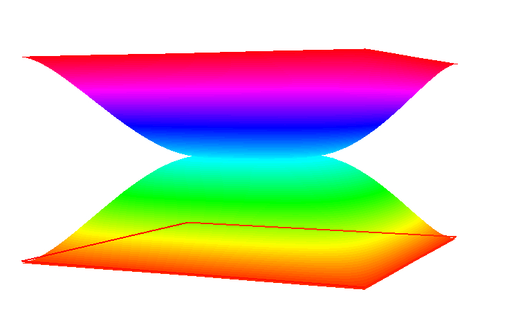
65 plot(ui1, ui2, wait=true, nbiso=60, dim=3);
66
67 if(iter > 1) break;
68
69 // Mesh adpatation
70 Th = adaptmesh(Th, [ui1, ui2], err=0.004, nbvx=100000);
71 [uz, uz2] = [uzi, uzi2];
72 [lz, lz2] = [lzi, lzi2];
73 [u1, u2] = [ui1, ui2];
74 lm = lmi;
75}
3D constrained minimum surface with IPOPT
Area and volume expressions
This example is aimed at numerically solving some constrained minimum surface problems with the IPOPT algorithm. We restrain to \(C^{k}\) (\(k\geq 1\)), closed, spherically parametrizable surfaces, i.e. surfaces \(S\) such that:
Where the components are expressed in the spherical coordinate system. Let’s call \(\Omega\) the \([0,2\pi ]\times[0,\pi]\) angular parameters set. In order to exclude self crossing and opened shapes, the following assumptions upon \(\rho\) are made:
For a given function \(\rho\) the first fundamental form (the metric) of the defined surface has the following matrix representation:
This metric is used to express the area of the surface. Let \(g=\det(G)\), then we have:
The volume of the space enclosed within the shape is easier to express:
Derivatives
In order to use a Newton based interior point optimization algorithm, one must be able to evaluate the derivatives of \(\mathcal{A}\) and \(\mathcal{V}\) with respect to \(rho\). Concerning the area, we have the following result:
Where \(\bar{g}\) is the application mapping the \((\theta,\phi) \mapsto g(\theta,\phi)\) scalar field to \(\rho\). This leads to the following expression, easy to transpose in a freefem script using:
With a similar approach, one can derive an expression for second order derivatives. However, comporting no specific difficulties, the detailed calculus are tedious, the result is that these derivatives can be written using a \(3\times 3\) matrix \(\mathbf{B}\) whose coefficients are expressed in term of \(\rho\) and its derivatives with respect to \(\theta\) and \(\phi\), such that:
Deriving the volume function derivatives is again an easier task. We immediately get the following expressions:
The problem and its script
The whole code is available in IPOPT minimal surface & volume example. We propose to solve the following problem:
Tip
Given a positive function \(\rho_{\mathrm{object}}\) piecewise continuous, and a scalar \(\mathcal{V}_{\mathrm{max}} > \mathcal{V}(\rho_{\mathrm{object}})\), find \(\rho_{0}\) such that:
If \(\rho_{\mathrm{object}}\) is the spherical parametrization of the surface of a 3-dimensional object (domain) \(\mathcal{O}\), it can be interpreted as finding the surface with minimum area enclosing the object with a given maximum volume. If \(\mathcal{V}_{\mathrm{max}}\) is close to \(\mathcal{V}(\rho_{\mathrm{object}})\), so should be \(\rho_{0}\) and \(\rho_{\mathrm{object}}\). With higher values of \(\mathcal{V}_{\mathrm{max}}\), \(\rho\) should be closer to the unconstrained minimum surface surrounding \(\mathcal{O}\) which is obtained as soon as \(\mathcal{V}_{\mathrm{max}} \geq \frac{4}{3}\pi \|\rho_{\mathrm{object}}\|_{\infty}^{3}\) (sufficient but not necessary).
It also could be interesting to solve the same problem with the constraint \(\mathcal{V}(\rho_{0})\geq \mathcal{V}_{\mathrm{min}}\) which leads to a sphere when \(\mathcal{V}_{\mathrm{min}} \geq \frac{1}{6}\pi \mathrm{diam}(\mathcal{O})^{3}\) and moves toward the solution of the unconstrained problem as \(\mathcal{V}_{\mathrm{min}}\) decreases.
We start by meshing the domain \([0,2\pi]\times\ [0,\pi]\), then a periodic P1 finite elements space is defined.
 1load "msh3";
 2load "medit";
 3load "ff-Ipopt";
 4
 5// Parameters
 6int nadapt = 3;
 7real alpha = 0.9;
 8int np = 30;
 9real regtest;
10int shapeswitch = 1;
11real sigma = 2*pi/40.;
12real treshold = 0.1;
13real e = 0.1;
14real r0 = 0.25;
15real rr = 2-r0;
16real E = 1./(e*e);
17real RR = 1./(rr*rr);
18
19// Mesh
20mesh Th = square(2*np, np, [2*pi*x, pi*y]);
21
22// Fespace
23fespace Vh(Th, P1, periodic=[[2, y], [4, y]]);
24//Initial shape definition
25//outside of the mesh adaptation loop to initialize with the previous optimial shape found on further iterations
26Vh startshape = 5;
We create some finite element functions whose underlying arrays will be used to store the values of dual variables associated to all the constraints in order to reinitialize the algorithm with it in the case where we use mesh adaptation. Doing so, the algorithm will almost restart at the accuracy level it reached before mesh adaptation, thus saving many iterations.
1Vh uz = 1., lz = 1.;
2rreal[int] lm = [1];
Then, follows the mesh adaptation loop, and a rendering function, Plot3D, using 3D mesh to display the shape it is passed with medit (the movemesh23 procedure often crashes when called with ragged shapes).
 1for(int kkk = 0; kkk < nadapt; ++kkk){
 2   int iter=0;
 3   func sin2 = square(sin(y));
 4
 5   // A function which transform Th in 3d mesh (r=rho)
 6   //a point (theta,phi) of Th becomes ( r(theta,phi)*cos(theta)*sin(phi) , r(theta,phi)*sin(theta)*sin(phi) , r(theta,phi)*cos(phi) )
 7   //then displays the resulting mesh with medit
 8   func int Plot3D (real[int] &rho, string cmm, bool ffplot){
 9      Vh rhoo;
10      rhoo[] = rho;
11      //mesh sTh = square(np, np/2, [2*pi*x, pi*y]);
12      //fespace sVh(sTh, P1);
13      //Vh rhoplot = rhoo;
14      try{
15         mesh3 Sphere = movemesh23(Th, transfo=[rhoo(x,y)*cos(x)*sin(y), rhoo(x,y)*sin(x)*sin(y), rhoo(x,y)*cos(y)]);
16         if(ffplot)
17            plot(Sphere);
18         else
19            medit(cmm, Sphere);
20      }
21      catch(...){
22         cout << "PLOT ERROR" << endl;
23      }
24      return 1;
25   }
26}
Here are the functions related to the area computation and its shape derivative, according to equations (31) and (33):
 1// Surface computation
 2//Maybe is it possible to use movemesh23 to have the surface function less complicated
 3//However, it would not simplify the gradient and the hessian
 4func real Area (real[int] &X){
 5   Vh rho;
 6   rho[] = X;
 7   Vh rho2 = square(rho);
 8   Vh rho4 = square(rho2);
 9   real res = int2d(Th)(sqrt(rho4*sin2 + rho2*square(dx(rho)) + rho2*sin2*square(dy(rho))));
10   ++iter;
11   if(1)
12      plot(rho, value=true, fill=true, cmm="rho(theta,phi) on [0,2pi]x[0,pi] - S="+res, dim=3);
13   else
14      Plot3D(rho[], "shape_evolution", 1);
15   return res;
16}
17
18func real[int] GradArea (real[int] &X){
19   Vh rho, rho2;
20   rho[] = X;
21   rho2[] = square(X);
22   Vh sqrtPsi, alpha;
23   {
24      Vh dxrho2 = dx(rho)*dx(rho), dyrho2 = dy(rho)*dy(rho);
25      sqrtPsi = sqrt(rho2*rho2*sin2 + rho2*dxrho2 + rho2*dyrho2*sin2);
26      alpha = 2.*rho2*rho*sin2 + rho*dxrho2 + rho*dyrho2*sin2;
27   }
28   varf dArea (u, v)
29      = int2d(Th)(
30           1./sqrtPsi * (alpha*v + rho2*dx(rho)*dx(v) + rho2*dy(rho)*sin2*dy(v))
31      )
32      ;
33
34   real[int] grad = dArea(0, Vh);
35   return grad;
36}
The function returning the hessian of the area for a given shape is a bit blurry, thus we won’t show here all of equation (34) coefficients definition, they can be found in the edp file.
 1matrix hessianA;
 2func matrix HessianArea (real[int] &X){
 3   Vh rho, rho2;
 4   rho[] = X;
 5   rho2 = square(rho);
 6   Vh sqrtPsi, sqrtPsi3, C00, C01, C02, C11, C12, C22, A;
 7   {
 8      Vh C0, C1, C2;
 9      Vh dxrho2 = dx(rho)*dx(rho), dyrho2 = dy(rho)*dy(rho);
10      sqrtPsi = sqrt( rho2*rho2*sin2 + rho2*dxrho2 + rho2*dyrho2*sin2);
11      sqrtPsi3 = (rho2*rho2*sin2 + rho2*dxrho2 + rho2*dyrho2*sin2)*sqrtPsi;
12      C0 = 2*rho2*rho*sin2 + rho*dxrho2 + rho*dyrho2*sin2;
13      C1 = rho2*dx(rho);
14      C2 = rho2*sin2*dy(rho);
15      C00 = square(C0);
16      C01 = C0*C1;
17      C02 = C0*C2;
18      C11 = square(C1);
19      C12 = C1*C2;
20      C22 = square(C2);
21      A = 6.*rho2*sin2 + dxrho2 + dyrho2*sin2;
22   }
23   varf d2Area (w, v)
24      =int2d(Th)(
25           1./sqrtPsi * (
26              A*w*v
27            + 2*rho*dx(rho)*dx(w)*v
28            + 2*rho*dx(rho)*w*dx(v)
29            + 2*rho*dy(rho)*sin2*dy(w)*v
30            + 2*rho*dy(rho)*sin2*w*dy(v)
31            + rho2*dx(w)*dx(v)
32            + rho2*sin2*dy(w)*dy(v)
33         )
34         + 1./sqrtPsi3 * (
35              C00*w*v
36            + C01*dx(w)*v
37            + C01*w*dx(v)
38            + C02*dy(w)*v
39            + C02*w*dy(v)
40            + C11*dx(w)*dx(v)
41            + C12*dx(w)*dy(v)
42            + C12*dy(w)*dx(v)
43            + C22*dy(w)*dy(v)
44         )
45      )
46      ;
47   hessianA = d2Area(Vh, Vh);
48   return hessianA;
49}
And the volume related functions:
 1// Volume computation
 2func real Volume (real[int] &X){
 3   Vh rho;
 4   rho[] = X;
 5   Vh rho3 = rho*rho*rho;
 6   real res = 1./3.*int2d(Th)(rho3*sin(y));
 7   return res;
 8}
 9
10func real[int] GradVolume (real[int] &X){
11   Vh rho;
12   rho[] = X;
13   varf dVolume(u, v) = int2d(Th)(rho*rho*sin(y)*v);
14   real[int] grad = dVolume(0, Vh);
15   return grad;
16}
17
18matrix hessianV;
19func matrix HessianVolume(real[int] &X){
20   Vh rho;
21   rho[] = X;
22   varf d2Volume(w, v) = int2d(Th)(2*rho*sin(y)*v*w);
23   hessianV = d2Volume(Vh, Vh);
24   return hessianV;
25}
If we want to use the volume as a constraint function we must wrap it and its derivatives in some FreeFEM functions returning the appropriate types. It is not done in the above functions in cases where one wants to use it as a fitness function. The lagrangian hessian also has to be wrapped since the Volume is not linear with respect to \(\rho\), it has some non-null second order derivatives.
1func real[int] ipVolume (real[int] &X){ real[int] vol = [Volume(X)]; return vol; }
2matrix mdV;
3func matrix ipGradVolume (real[int] &X) { real[int,int] dvol(1,Vh.ndof); dvol(0,:) = GradVolume(X); mdV = dvol; return mdV; }
4matrix HLagrangian;
5func matrix ipHessianLag (real[int] &X, real objfact, real[int] &lambda){
6   HLagrangian = objfact*HessianArea(X) + lambda[0]*HessianVolume(X);
7   return HLagrangian;
8}
The ipGradVolume function could pose some troubles during the optimization process because the gradient vector is transformed in a sparse matrix, so any null coefficient will be discarded.
Here we create the IPOPT structure manually and use the checkindex named-parameter to avoid bad indexing during copies.
This gradient is actually dense, there is no reason for some components to be constantly zero:
1int[int] gvi(Vh.ndof), gvj=0:Vh.ndof-1;
2gvi = 0;
These two arrays will be passed to IPOPT with structjacc=[gvi,gvj].
The last remaining things are the bound definitions.
The simple lower bound must be equal to the components of the P1 projection of \(\rho_{object}\).
And we choose \(\alpha\in [0,1]\) to set \(\mathcal{V}_{\mathrm{max}}\) to \((1-\alpha) \mathcal{V}(\rho_{object}) + \alpha\frac{4}{3}\pi \|\rho_{\mathrm{object}}\|_{\infty}^{3}\):
 1func disc1 = sqrt(1./(RR+(E-RR)*cos(y)*cos(y)))*(1+0.1*cos(7*x));
 2func disc2 = sqrt(1./(RR+(E-RR)*cos(x)*cos(x)*sin2));
 3
 4if(1){
 5   lb = r0;
 6   for (int q = 0; q < 5; ++q){
 7      func f = rr*Gaussian(x, y, 2*q*pi/5., pi/3.);
 8      func g = rr*Gaussian(x, y, 2*q*pi/5.+pi/5., 2.*pi/3.);
 9      lb = max(max(lb, f), g);
10   }
11   lb = max(lb, rr*Gaussian(x, y, 2*pi, pi/3));
12}
13lb = max(lb, max(disc1, disc2));
14real Vobj = Volume(lb[]);
15real Vnvc = 4./3.*pi*pow(lb[].linfty,3);
16
17if(1)
18   Plot3D(lb[], "object_inside", 1);
19real[int] clb = 0., cub = [(1-alpha)*Vobj + alpha*Vnvc];
Calling IPOPT:
1int res = IPOPT(Area, GradArea, ipHessianLag, ipVolume, ipGradVolume,
2   rc[], ub=ub[], lb=lb[], clb=clb, cub=cub, checkindex=1, maxiter=kkk<nadapt-1 ? 40:150,
3   warmstart=kkk, lm=lm, uz=uz[], lz=lz[], tol=0.00001, structjacc=[gvi,gvj]);
4cout << "IPOPT: res =" << res << endl ;
5
6// Plot
7Plot3D(rc[], "Shape_at_"+kkk, 1);
8Plot3D(GradArea(rc[]), "ShapeGradient", 1);
Finally, before closing the mesh adaptation loop, we have to perform the said adaptation. The mesh is adaptated with respect to the \(X=(\rho, 0, 0)\) (in spherical coordinates) vector field, not directly with respect to \(\rho\), otherwise the true curvature of the 3D-shape would not be well taken into account.
1if (kkk < nadapt-1){
2   Th = adaptmesh(Th, rc*cos(x)*sin(y), rc*sin(x)*sin(y), rc*cos(y),
3      nbvx=50000, periodic=[[2, y], [4, y]]);
4   plot(Th, wait=true);
5   startshape = rc;
6   uz = uz;
7   lz = lz;
8}
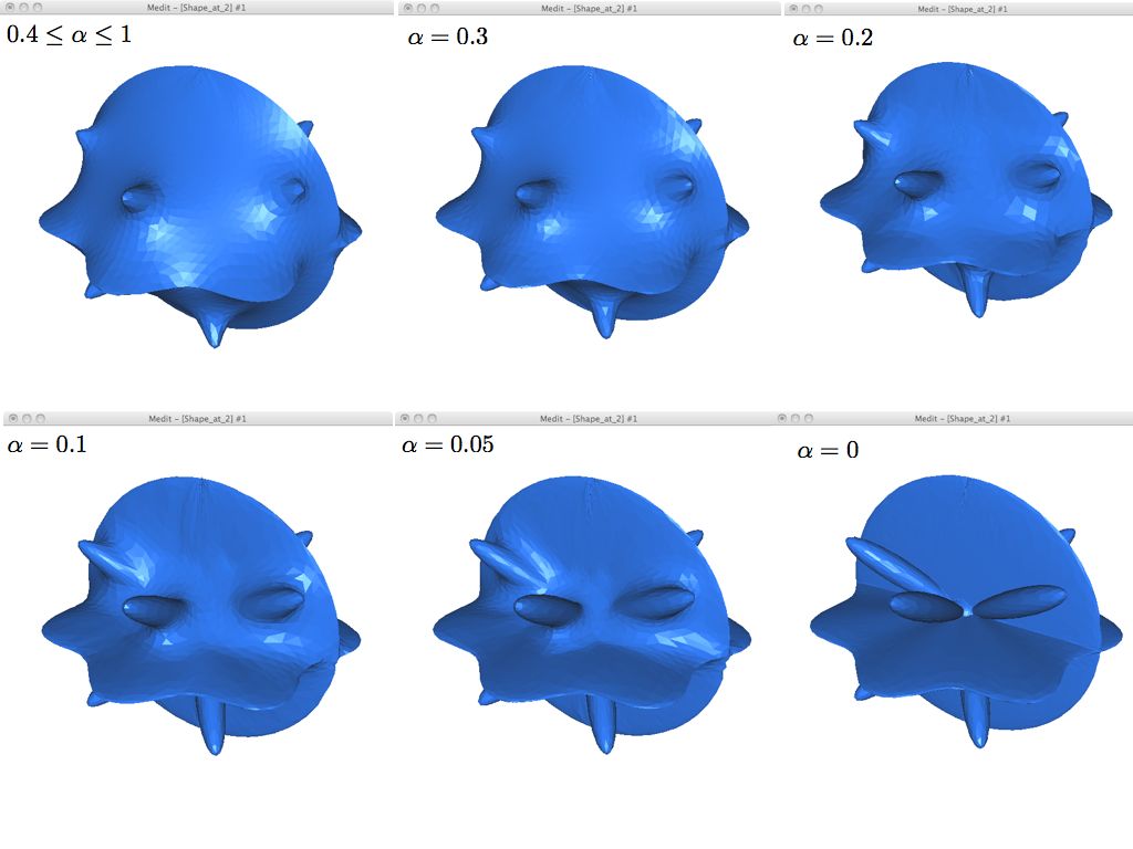
Here are some pictures of the resulting surfaces obtained for decreasing values of \(\alpha\) (and a slightly more complicated object than two orthogonal discs). We return to the enclosed object when \(\alpha=0\):
The nlOpt optimizers
The ff-NLopt package provides a FreeFEM interface to the free/open-source library for nonlinear optimization, easing the use of several different free optimization (constrained or not) routines available online along with the PDE solver.
All the algorithms are well documented in NLopt documentation, therefore no exhaustive information concerning their mathematical specificities will be found here and we will focus on the way they are used in a FreeFEM script.
If needing detailed information about these algorithms, visit the website where a description of each of them is given, as well as many bibliographical links.
Most of the gradient based algorithms of NLopt uses a full matrix approximation of the Hessian, so if you’re planning to solve a large scale problem, use the IPOPT optimizer which definitely surpass them.
All the NLopt features are identified that way:
 1load "ff-NLopt"
 2//define J, u, and maybe grad(J), some constraints etc...
 3real min = nloptXXXXXX(J, u, //Unavoidable part
 4   grad=<name of grad(J)>, //if needed
 5   lb= //Lower bounds array
 6   ub= //Upper bounds array
 7   ... //Some optional arguments:
 8   //Constraints functions names,
 9   //Stopping criteria,
10   //Algorithm specific parameters,
11   //Etc...
12);
XXXXXX refers to the algorithm tag (not necessarily 6 characters long).
u is the starting position (a real[int] type array) which will be overwritten by the algorithm, the value at the end being the found \(argmin\).
And as usual, J is a function taking a real[int] type array as argument and returning a real.
grad, lb and ub are “half-optional” arguments, in the sense that they are obligatory for some routines but not all.
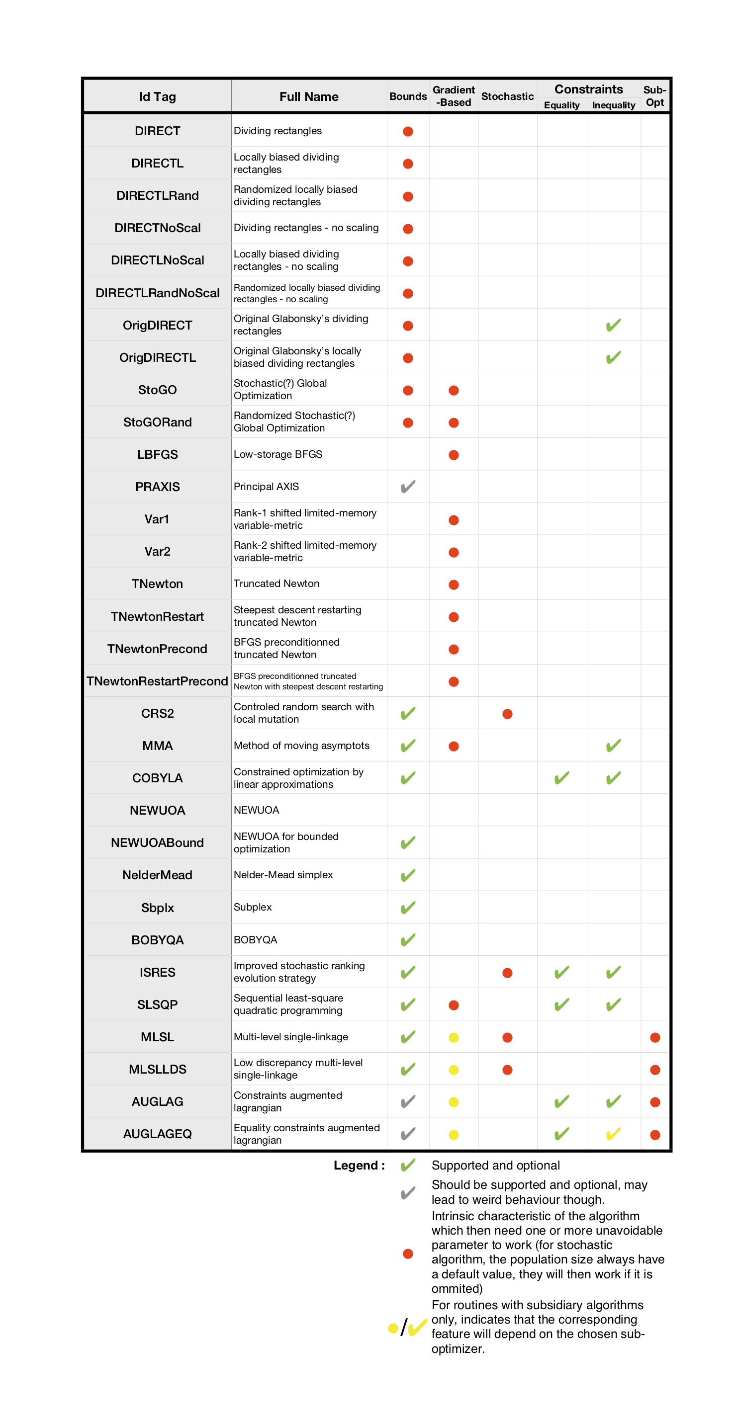
The possible optionally named parameters are the following, note that they are not used by all algorithms (some do not support constraints, or a type of constraints, some are gradient-based and others are derivative free, etc…). One can refer to the table after the parameters description to check which are the named parameters supported by a specific algorithm. Using an unsupported parameter will not stop the compiler work, seldom breaks runtime, and will just be ignored. When it is obvious you are missing a routine, you will get a warning message at runtime (for example if you pass a gradient to a derivative free algorithm, or set the population of a non-genetic one, etc…). In the following description, \(n\) stands for the dimension of the search space.
Half-optional parameters :
grad=The name of the function which computes the gradient of the cost function (prototype should bereal[int]\(\rightarrow\)real[int], both argument and result should have the size \(n\)). This is needed as soon as a gradient-based method is involved, which is ignored if defined in a derivative free context.lb/ub= Lower and upper bounds arrays (real[int]type) of size \(n\). Used to define the bounds within which the search variable is allowed to move. Needed for some algorithms, optional, or unsupported for others.subOpt: Only enabled for the Augmented Lagrangian and MLSL methods who need a sub-optimizer in order to work. Just pass the tag of the desired local algorithm with astring.
Constraints related parameters (optional - unused if not specified):
IConst/EConst: Allows to pass the name of a function implementing some inequality (resp. equality) constraints on the search space. The function type must bereal[int]\(\rightarrow\)real[int]where the size of the returned array is equal to the number of constraints (of the same type - it means that all of the constraints are computed in one vectorial function). In order to mix inequality and equality constraints in a same minimization attempt, two vectorial functions have to be defined and passed. See example (36) for more details about how these constraints have to be implemented.gradIConst/gradEConst: Use to provide the inequality (resp. equality) constraints gradient. These arereal[int]\(\rightarrow\)real[int,int]type functions. Assuming we have defined a constraint function (either inequality or equality) with \(p\) constraints, the size of the matrix returned by its associated gradient must be \(p\times n\) (the \(i\)-th line of the matrix is the gradient of the \(i\)-th constraint). It is needed in a gradient-based context as soon as an inequality or equality constraint function is passed to the optimizer and ignored in all other cases.tolIConst/tolEConst: Tolerance values for each constraint. This is an array of size equal to the number of inequality (resp. equality) constraints. Default value is set to \(10^{-12}\) for each constraint of any type.
Stopping criteria :
stopFuncValue: Makes the algorithm end when the objective function reaches thisrealvalue.stopRelXTol: Stops the algorithm when the relative moves in each direction of the search space is smaller than thisrealvalue.stopAbsXTol: Stops the algorithm when the moves in each direction of the search space is smaller than the corresponding value in thisreal[int]array.stopRelFTol: Stops the algorithm when the relative variation of the objective function is smaller than thisrealvalue.stopAbsFTol: Stops the algorithm when the variation of the objective function is smaller than thisrealvalue.stopMaxFEval: Stops the algorithm when the number of fitness evaluations reaches thisintegervalue.stopTime: Stops the algorithm when the optimization time in seconds exceeds thisrealvalue. This is not a strict maximum: the time may exceed it slightly, depending upon the algorithm and on how slow your function evaluation is.Note that when an AUGLAG or MLSL method is used, the meta-algorithm and the sub-algorithm may have different termination criteria. Thus, for algorithms of this kind, the following named parameters has been defined (just adding the SO prefix - for Sub-Optimizer) to set the ending condition of the sub-algorithm (the meta one uses the ones above):
SOStopFuncValue,SOStopRelXTol, and so on… If these are not used, the sub-optimizer will use those of the master routine.
Other named parameters :
popSize:integerused to change the size of the sample for stochastic search methods. Default value is a peculiar heuristic to the chosen algorithm.SOPopSize: Same as above, but when the stochastic search is passed to a meta-algorithm.nGradStored: The number (integertype) of gradients to “remember” from previous optimization steps: increasing this increases the memory requirements but may speed convergence. It is set to a heuristic value by default. If used with AUGLAG or MLSL, it will only affect the given subsidiary algorithm.
The following table sums up the main characteristics of each algorithm, providing the more important information about which features are supported by which algorithm and what are the unavoidable arguments they need. More details can be found in NLopt documentation.
Tip
Variational inequality
Let \(\Omega\) be a domain of \(\mathbb{R}^{2}\), \(f_{1}, f_{2}\in L^{2}(\Omega)\) and \(g_{1}, g_{2} \in L^{2}(\partial\Omega)\) four given functions with \(g_{1}\leq g_{2}\) almost everywhere.
We define the space:
as well as the function \(J:H^{1}(\Omega)^{2}\longrightarrow \mathbb{R}\):
The problem consists in finding (numerically) two functions \((u_{1},u_{2}) = \underset{(v_{1},v_{2})\in V}{\operatorname{argmin}} J(v_{1},v_{2})\).
This can be interpreted as finding \(u_{1}, u_{2}\) as close as possible (in a certain sense) to the solutions of the Laplace equation with respectively \(f_{1}, f_{2}\) second members and \(g_{1}, g_{2}\) Dirichlet boundary conditions with the \(u_{1}\leq u_{2}\) almost everywhere constraint.
Here is the corresponding script to treat this variational inequality problem with one of the NLOpt algorithms.
1//A brief script to demonstrate how to use the freefemm interfaced nlopt routines
2//The problem consist in solving a simple variational inequality using one of the
3//optimization algorithm of nlopt. We restart the algorithlm a few times after
4//performing some mesh adaptation to get a more precise output
5
6load "ff-NLopt"
7
8// Parameters
9int kas = 3; //choose of the algorithm
10int NN = 10;
11func f1 = 1.;
12func f2 = -1.;
13func g1 = 0.;
14func g2 = 0.1;
15int iter = 0;
16int nadapt = 2;
17real starttol = 1e-6;
18real bctol = 6.e-12;
19
20// Mesh
21mesh Th = square(NN, NN);
22
23// Fespace
24fespace Vh(Th, P1);
25Vh oldu1, oldu2;
26
27// Adaptation loop
28for (int al = 0; al < nadapt; ++al){
29 varf BVF (v, w) = int2d(Th)(0.5*dx(v)*dx(w) + 0.5*dy(v)*dy(w));
30 varf LVF1 (v, w) = int2d(Th)(f1*w);
31 varf LVF2 (v, w) = int2d(Th)(f2*w);
32 matrix A = BVF(Vh, Vh);
33 real[int] b1 = LVF1(0, Vh), b2 = LVF2(0, Vh);
34
35 varf Vbord (v, w) = on(1, 2, 3, 4, v=1);
36
37 Vh In, Bord;
38 Bord[] = Vbord(0, Vh, tgv=1);
39 In[] = Bord[] ? 0:1;
40 Vh gh1 = Bord*g1, gh2 = Bord*g2;
41
42 func real J (real[int] &X){
43 Vh u1, u2;
44 u1[] = X(0:Vh.ndof-1);
45 u2[] = X(Vh.ndof:2*Vh.ndof-1);
46 iter++;
47 real[int] Au1 = A*u1[], Au2 = A*u2[];
48 Au1 -= b1;
49 Au2 -= b2;
50 real val = u1[]'*Au1 + u2[]'*Au2;
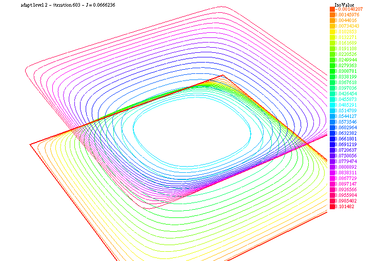
51 if (iter%10 == 9)
52 plot(u1, u2, nbiso=30, fill=1, dim=3, cmm="adapt level "+al+" - iteration "+iter+" - J = "+val, value=1);
53 return val;
54 }
55
56 varf dBFV (v, w) = int2d(Th)(dx(v)*dx(w)+dy(v)*dy(w));
57 matrix dA = dBFV(Vh, Vh);
58 func real[int] dJ (real[int] &X){
59 Vh u1, u2;
60 u1[] = X(0:Vh.ndof-1);
61 u2[] = X(Vh.ndof:2*Vh.ndof-1);
62
63 real[int] grad1 = dA*u1[], grad2 = dA*u2[];
64 grad1 -= b1;
65 grad2 -= b2;
66 real[int] Grad(X.n);
67 Grad(0:Vh.ndof-1) = grad1;
68 Grad(Vh.ndof:2*Vh.ndof-1) = grad2;
69 return Grad;
70 }
71
72 func real[int] IneqC (real[int] &X){
73 real[int] constraints(Vh.ndof);
74 for (int i = 0; i < Vh.ndof; ++i) constraints[i] = X[i] - X[i+Vh.ndof];
75 return constraints;
76 }
77
78 func real[int,int] dIneqC (real[int] &X){
79 real[int, int] dconst(Vh.ndof, 2*Vh.ndof);
80 dconst = 0;
81 for(int i = 0; i < Vh.ndof; ++i){
82 dconst(i, i) = 1.;
83 dconst(i, i+Vh.ndof) = -1.;
84 }
85 return dconst;
86 }
87
88 real[int] BordIndex(Th.nbe); //Indexes of border d.f.
89 {
90 int k = 0;
91 for (int i = 0; i < Bord.n; ++i) if (Bord[][i]){ BordIndex[k] = i; ++k; }
92 }
93
94 func real[int] BC (real[int] &X){
95 real[int] bc(2*Th.nbe);
96 for (int i = 0; i < Th.nbe; ++i){
97 int I = BordIndex[i];
98 bc[i] = X[I] - gh1[][I];
99 bc[i+Th.nbe] = X[I+Th.nv] - gh2[][I];
100 }
101 return bc;
102 }
103
104 func real[int, int] dBC(real[int] &X){
105 real[int, int] dbc(2*Th.nbe,2*Th.nv);
106 dbc = 0.;
107 for (int i = 0; i < Th.nbe; ++i){
108 int I = BordIndex[i];
109 dbc(i, I) = 1.;
110 dbc(i+Th.nbe, I+Th.nv) = 1.;
111 }
112 return dbc;
113 }
114
115 real[int] start(2*Vh.ndof), up(2*Vh.ndof), lo(2*Vh.ndof);
116
117 if (al == 0){
118 start(0:Vh.ndof-1) = 0.;
119 start(Vh.ndof:2*Vh.ndof-1) = 0.01;
120 }
121 else{
122 start(0:Vh.ndof-1) = oldu1[];
123 start(Vh.ndof:2*Vh.ndof-1) = oldu2[];
124 }
125
126 up = 1000000;
127 lo = -1000000;
128 for (int i = 0; i < Vh.ndof; ++i){
129 if (Bord[][i]){
130 up[i] = gh1[][i] + bctol;
131 lo[i] = gh1[][i] - bctol;
132 up[i+Vh.ndof] = gh2[][i] + bctol;
133 lo[i+Vh.ndof] = gh2[][i] - bctol;
134 }
135 }
136
137 real mini = 1e100;
138 if (kas == 1)
139 mini = nloptAUGLAG(J, start, grad=dJ, lb=lo,
140 ub=up, IConst=IneqC, gradIConst=dIneqC,
141 subOpt="LBFGS", stopMaxFEval=10000, stopAbsFTol=starttol);
142 else if (kas == 2)
143 mini = nloptMMA(J, start, grad=dJ, lb=lo, ub=up, stopMaxFEval=10000, stopAbsFTol=starttol);
144 else if (kas == 3)
145 mini = nloptAUGLAG(J, start, grad=dJ, IConst=IneqC,
146 gradIConst=dIneqC, EConst=BC, gradEConst=dBC,
147 subOpt="LBFGS", stopMaxFEval=200, stopRelXTol=1e-2);
148 else if (kas == 4)
149 mini = nloptSLSQP(J, start, grad=dJ, IConst=IneqC,
150 gradIConst=dIneqC, EConst=BC, gradEConst=dBC,
151 stopMaxFEval=10000, stopAbsFTol=starttol);
152 Vh best1, best2;
153 best1[] = start(0:Vh.ndof-1);
154 best2[] = start(Vh.ndof:2*Vh.ndof-1);
155
156 Th = adaptmesh(Th, best1, best2);
157 oldu1 = best1;
158 oldu2 = best2;
159}
Optimization with MPI
The only quick way to use the previously presented algorithms on a parallel architecture lies in parallelizing the used cost function (which is in most real life cases, the expensive part of the algorithm). Somehow, we provide a parallel version of the CMA-ES algorithm. The parallelization principle is the trivial one of evolving/genetic algorithms: at each iteration the cost function has to be evaluated \(N\) times without any dependence at all, these \(N\) calculus are then equally distributed to each process. Calling the MPI version of CMA-ES is nearly the same as calling its sequential version (a complete example of use can be found in the CMAES MPI variational inequality example):
1load "mpi-cmaes"
2... // Define J, u and all here
3real min = cmaesMPI(J, u, stopTolFun=1e-6, stopMaxIter=3000);
4cout << "minimum value is " << min << " for u = " << u << endl;
If the population size is not changed using the popsize parameter, it will use the heuristic value slightly changed to be equal to the closest greatest multiple of the size of the communicator used by the optimizer.
The FreeFEM mpicommworld is used by default.
The user can specify his own MPI communicator with the named parameter comm=, see the MPI section of this manual for more information about communicators in FreeFEM.