Elasticity

Consider an elastic plate with undeformed shape \(\Omega\times ]-h,h[\) in \(\mathbb{R}^3\), \(\Omega\subset\mathbb{R}^2\).

By the deformation of the plate, we assume that a point \(P(x_1,x_2,x_3)\) moves to \({\cal P}(\xi_1,\xi_2,\xi_3)\). The vector \(\mathbf{u}=(u_1,u_2,u_3)=(\xi_1-x_1,\xi_2-x_2,\xi_3-x_3)\) is called the displacement vector.

By the deformation, the line segment \(\overline{\mathbf{x},\mathbf{x}+\tau\Delta\mathbf{x}}\) moves approximately to \(\overline{\mathbf{x}+\mathbf{u}(\mathbf{x}),\mathbf{x}+\tau\Delta\mathbf{x} +\mathbf{u}(\mathbf{x}+\tau\Delta\mathbf{x})}\) for small \(\tau\), where \(\mathbf{x}=(x_1,x_2,x_3),\, \Delta\mathbf{x} =(\Delta x_1,\Delta x_2,\Delta x_3)\).

We now calculate the ratio between two segments:

\[\eta(\tau)=\tau^{-1}|\Delta\mathbf{x}|^{-1} \left(|\mathbf{u}(\mathbf{x}+\tau\Delta\mathbf{x}) -\mathbf{u}(\mathbf{x})+\tau\Delta\mathbf{x}|-\tau|\Delta\mathbf{x}|\right)\]

then we have (see e.g. [NECAS2017], p.32)

\[\lim_{\tau\to 0}\eta(\tau)=(1+2e_{ij}\nu_i\nu_j)^{1/2}-1, \quad 2e_{ij}=\frac{\partial u_k}{\partial x_i}\frac{\partial u_k}{\partial x_j}+\left(\frac{\partial u_i}{\partial x_j}+ \frac{\partial u_j}{\partial x_i}\right)\]

where \(\nu_i=\Delta x_i|\Delta\mathbf{x}|^{-1}\). If the deformation is small, then we may consider that:

\[(\partial u_k/\partial x_i)(\partial u_k/\partial x_i)\approx 0\]

and the following is called small strain tensor:

\[\varepsilon_{ij}(u)=\frac{1}{2}\left(\frac{\partial u_i}{\partial x_j}+ \frac{\partial u_j}{\partial x_i}\right)\]

The tensor \(e_{ij}\) is called finite strain tensor.

Consider the small plane \(\Delta \Pi(\mathbf{x})\) centered at \(\mathbf{x}\) with the unit normal direction \(\mathbf{n}=(n_1,n_2,n_3)\), then the surface on \(\Delta \Pi(\mathbf{x})\) at \(\mathbf{x}\) is:

\[(\sigma_{1j}(\mathbf{x})n_j, \sigma_{2j}(\mathbf{x})n_j, \sigma_{3j}(\mathbf{x})n_j)\]

where \(\sigma_{ij}(\mathbf{x})\) is called stress tensor at \(\mathbf{x}\). Hooke’s law is the assumption of a linear relation between \(\sigma_{ij}\) and \(\varepsilon_{ij}\) such as:

\[\sigma_{ij}(\mathbf{x})=c_{ijkl}(\mathbf{x})\varepsilon_{ij}(\mathbf{x})\]

with the symmetry \(c_{ijkl}=c_{jikl}, c_{ijkl}=c_{ijlk}, c_{ijkl}=c_{klij}\).

If Hooke’s tensor \(c_{ijkl}(\mathbf{x})\) do not depend on the choice of coordinate system, the material is called isotropic at \(\mathbf{x}\).

If \(c_{ijkl}\) is constant, the material is called homogeneous. In homogeneous isotropic case, there is Lamé constants \(\lambda, \mu\) (see e.g. [NECAS2017], p.43) satisfying

\[\sigma_{ij}=\lambda\delta_{ij}\textrm{div}\mathbf{u}+2\mu \varepsilon_{ij}\]

where \(\delta_{ij}\) is Kronecker’s delta.

We assume that the elastic plate is fixed on \(\Gamma_D\times ]-h,h[,\, \Gamma_D\subset \partial\Omega\). If the body force \(\mathbf{f}=(f_1,f_2,f_3)\) is given in \(\Omega\times]-h,h[\) and surface force \(\mathbf{g}\) is given in \(\Gamma_N\times]-h,h[, \Gamma_N=\partial\Omega\setminus\overline{\Gamma_D}\), then the equation of equilibrium is given as follows:

(58)\[\begin{split}\begin{array}{rcl} -\partial_j \sigma_{ij}&=&f_i~~\textrm{in }\Omega\times ]-h,h[,\quad i=1,2,3\\ \sigma_{ij}n_j&=&g_i~~\textrm{on }\Gamma_N\times ]-h,h[,\quad u_i=0~~\textrm{on }\Gamma_D\times ]-h,h[,\quad i=1,2,3 \end{array}\end{split}\]

We now explain the plain elasticity.

Plain strain:

On the end of plate, the contact condition \(u_3=0,\, g_3=\) is satisfied.

In this case, we can suppose that \(f_3=g_3=u_3=0\) and \(\mathbf{u}(x_1,x_2,x_3)=\overline{u}(x_1,x_2)\) for all \(-h<x_3<h\).
Plain stress:

The cylinder is assumed to be very thin and subjected to no load on the ends \(x_3=\pm h\), that is,

\[\sigma_{3i}=0,\quad x_3=\pm h,\quad i~1,2,3\]

The assumption leads that \(\sigma_{3i}=0\) in \(\Omega\times ]-h,h[\) and \(\mathbf{u}(x_1,x_2,x_3)=\overline{u}(x_1,x_2)\) for all \(-h<x_3<h\).
Generalized plain stress:

The cylinder is subjected to no load at \(x_3=\pm h\). Introducing the mean values with respect to thickness,

\[\overline{u}_i(x_1,x_2)=\frac{1}{2h}\int_{-h}^h{u(x_1,x_2,x_3)dx_3}\]

and we derive \(\overline{u}_3\equiv 0\). Similarly we define the mean values \(\overline{f},\overline{g}\) of the body force and surface force as well as the mean values \(\overline{\varepsilon}_{ij}\) and \(\overline{\sigma}_{ij}\) of the components of stress and strain, respectively.

In what follows we omit the overlines of \(\overline{u}, \overline{f},\overline{g}, \overline{\varepsilon}_{ij}\) and \(\overline{\varepsilon}_{ij}\). Then we obtain similar equation of equilibrium given in (58) replacing \(\Omega\times ]-h,h[\) with \(\Omega\) and changing \(i=1,2\). In the case of plane stress, \(\sigma_{ij}=\lambda^* \delta_{ij}\textrm{div}u+2\mu\varepsilon_{ij}, \lambda^*=(2\lambda \mu)/(\lambda+\mu)\).

The equations of elasticity are naturally written in variational form for the displacement vector \(\mathbf{u}(\mathbf{x})\in V\) as:

\[\int_\Omega [2\mu\epsilon_{ij}(\mathbf{u})\epsilon_{ij}(\mathbf{v}) +\lambda \epsilon_{ii}(\mathbf{u})\epsilon_{jj}(\mathbf{v})] =\int_\Omega \mathbf{f}\cdot \mathbf{v} +\int_\Gamma \mathbf{g}\cdot \mathbf{v}, \forall \mathbf{v}\in V\]

where \(V\) is the linear closed subspace of \(H^1(\Omega)^2\).

Tip

Beam

Consider an elastic plate with the undeformed rectangle shape \(]0,10[\times ]0,2[\). The body force is the gravity force \(\mathbf{f}\) and the boundary force \(\mathbf{g}\) is zero on lower and upper side. On the two vertical sides of the beam are fixed.

// Parameters
real E = 21.5;
real sigma = 0.29;
real gravity = -0.05;

// Mesh
border a(t=2, 0){x=0; y=t; label=1;}
border b(t=0, 10){x=t; y=0; label=2;}
border c(t=0, 2){ x=10; y=t; label=1;}
border d(t=0, 10){ x=10-t; y=2; label=3;}
mesh th = buildmesh(b(20) + c(5) + d(20) + a(5));

// Fespace
fespace Vh(th, [P1, P1]);
Vh [uu, vv];
Vh [w, s];

// Macro
real sqrt2 = sqrt(2.);
macro epsilon(u1, u2) [dx(u1), dy(u2), (dy(u1)+dx(u2))/sqrt2] //
macro div(u,v) (dx(u) + dy(v)) //

// Problem
real mu = E/(2*(1+sigma));
real lambda = E*sigma/((1+sigma)*(1-2*sigma));
solve Elasticity ([uu, vv], [w, s])
    = int2d(th)(
          lambda*div(w,s)*div(uu,vv)
        + 2.*mu*( epsilon(w,s)'*epsilon(uu,vv) )
    )
    + int2d(th)(
        - gravity*s
    )
    + on(1, uu=0, vv=0)
;

// Plot
plot([uu, vv], wait=true);
plot([uu,vv], wait=true, bb=[[-0.5, 2.5], [2.5, -0.5]]);

// Movemesh
mesh th1 = movemesh(th, [x+uu, y+vv]);
plot(th1, wait=true);

Tip

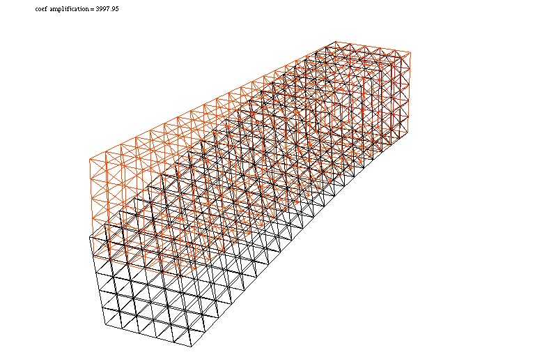
Beam 3D

Consider elastic box with the undeformed parallelepiped shape \(]0,5[\times ]0,1[\times]0,1[\). The body force is the gravity force \(\mathbf{f}\) and the boundary force \(\mathbf{g}\) is zero on all face except one the one vertical left face where the beam is fixed.

include "cube.idp"

// Parameters
int[int] Nxyz = [20, 5, 5];
real [int, int] Bxyz = [[0., 5.], [0., 1.], [0., 1.]];
int [int, int] Lxyz = [[1, 2], [2, 2], [2, 2]];

real E = 21.5e4;
real sigma = 0.29;
real gravity = -0.05;

// Mesh
mesh3 Th = Cube(Nxyz, Bxyz, Lxyz);

// Fespace
fespace Vh(Th, [P1, P1, P1]);
Vh [u1, u2, u3], [v1, v2, v3];

// Macro
real sqrt2 = sqrt(2.);
macro epsilon(u1, u2, u3) [
    dx(u1), dy(u2), dz(u3),
    (dz(u2) + dy(u3))/sqrt2,
    (dz(u1) + dx(u3))/sqrt2,
    (dy(u1) + dx(u2))/sqrt2] //
macro div(u1, u2, u3) (dx(u1) + dy(u2) + dz(u3)) //

// Problem
real mu = E/(2*(1+sigma));
real lambda = E*sigma/((1+sigma)*(1-2*sigma));

solve Lame ([u1, u2, u3], [v1, v2, v3])
    = int3d(Th)(
          lambda*div(u1, u2, u3)*div(v1, v2, v3)
        + 2.*mu*( epsilon(u1, u2, u3)'*epsilon(v1, v2, v3) )
    )
    - int3d(Th)(
          gravity*v3
    )
    + on(1, u1=0, u2=0, u3=0)
    ;

// Display
real dmax = u1[].max;
cout << "max displacement = " << dmax << endl;

// Movemesh
real coef = 0.1/dmax;
int[int] ref2 = [1, 0, 2, 0];
mesh3 Thm = movemesh3(Th, transfo=[x+u1*coef, y+u2*coef, z+u3*coef], label=ref2);
Thm = change(Thm, label=ref2);

// Plot
plot(Th, Thm, wait=true, cmm="coef amplification = "+coef);

../_images/Elasticity_Beam3D.jpg — Fig. 150 3d Beam deformed and undeformed box

Fracture Mechanics

Consider the plate with the crack whose undeformed shape is a curve \(\Sigma\) with the two edges \(\gamma_1,\, \gamma_2\).

We assume the stress tensor \(\sigma_{ij}\) is the state of plate stress regarding \((x,y)\in \Omega_{\Sigma}=\Omega\setminus \Sigma\). Here \(\Omega\) stands for the undeformed shape of elastic plate without crack.

If the part \(\Gamma_N\) of the boundary \(\partial\Omega\) is fixed and a load \({\cal L}=(\mathbf{f},\mathbf{g})\in L^2(\Omega)^2\times L^2(\Gamma_N)^2\) is given, then the displacement \(\mathbf{u}\) is the minimizer of the potential energy functional:

\[{\cal E}(\mathbf{v};{\cal L},\Omega_{\Sigma}) =\int_{\Omega_{\Sigma}} \{w(x,\mathbf{v})-\mathbf{f}\cdot \mathbf{v}\} -\int_{\Gamma_N}\mathbf{g}\cdot \mathbf{v}\]

over the functional space \(V(\Omega_{\Sigma})\),

\[V(\Omega_{\Sigma}) =\left\{ \mathbf{v}\in H^1(\Omega_{\Sigma})^2;\; \mathbf{v}=0\quad \hbox{ on } \Gamma_D=\partial\Omega\setminus\overline{\Gamma_N}\right\},\]

where \(w(x,\mathbf{v})=\sigma_{ij}(\mathbf{v})\varepsilon_{ij}(\mathbf{v})/2\),

\[\sigma_{ij}(\mathbf{v})=C_{ijkl}(x)\varepsilon_{kl}(\mathbf{v}),\quad \varepsilon_{ij}(\mathbf{v})=(\partial v_i/\partial x_j+ \partial v_j/\partial x_i)/2, \qquad (C_{ijkl}:\quad \hbox{Hooke's tensor}).\]

If the elasticity is homogeneous isotropic, then the displacement \(\mathbf{u}(x)\) is decomposed in an open neighborhood \(U_k\) of \(\gamma_k\) as in (see e.g. [OHTSUKA2000])

(59)\[\mathbf{u}(x) = \sum_{l=1}^2 K_l(\gamma_k) r_k^{1/2} S^C_{kl}(\theta_k) + \mathbf{u}_{k,R}(x) \quad \mbox{for }x\in \Omega_{\Sigma}\cap U_k,\, k=1,2\]

with \(\mathbf{u}_{k,R} \in H^2(\Omega_\Sigma\cap U_k)^2\), where \(U_k,\, k=1,2\) are open neighborhoods of \(\gamma_k\) such that \(\partial L_1\cap U_1=\gamma_1,\, \partial L_m\cap U_2=\gamma_2\), and

\[\begin{split}\begin{array}{rcl} S^C_{k1}(\theta_k) & = & \frac 1 {4\mu} \frac 1 {(2\pi)^{1/2}} \left[ \begin{array}{c} [2\kappa-1]\cos(\theta_k/2)-\cos(3\theta_k/2)\\ -[2\kappa+1]\sin(\theta_k/2)+\sin(3\theta_k/2) \end{array}\right],\\ S^C_{k2}(\theta_k) & = & \frac 1 {4\mu} \frac 1 {(2\pi)^{1/2}} \left[ \begin{array}{c} -[2\kappa-1]\sin(\theta_k/2)+3\sin(3\theta_k/2)\\ -[2\kappa+1]\cos(\theta_k/2)+\cos(3\theta_k/2) \end{array}\right]. \nonumber \end{array}\end{split}\]

where \(\mu\) is the shear modulus of elasticity, \(\kappa=3-4\nu\) (\(\nu\) is the Poisson’s ratio) for plane strain and \(\kappa=\frac {3-\nu} {1+\nu}\) for plane stress.

The coefficients \(K_1(\gamma_i)\) and \(K_2(\gamma_i),\) which are important parameters in fracture mechanics, are called stress intensity factors of the opening mode (mode I) and the sliding mode (mode II), respectively.

For simplicity, we consider the following simple crack

\[\Omega=\{(x,y):\; -1<x<1, -1<y<1\},\qquad \Sigma=\{(x,y):\; -1\le x\le 0, y=0\}\]

with only one crack tip \(\gamma=(0,0)\). Unfortunately, FreeFEM cannot treat crack, so we use the modification of the domain with U-shape channel (see U-shape example, Fig. 85) with \(d=0.0001\). The undeformed crack \(\Sigma\) is approximated by

\[\Sigma_d = \{(x,y):\; -1\le x\le -10*d, -d\le y\le d\} \cup\{(x,y):\; -10*d\le x\le 0, -d+0.1*x\le y\le d-0.1*x\}\]

and \(\Gamma_D=\)R in U-shape example, Fig. 85.

In this example, we use three technique:

Fast Finite Element Interpolator from the mesh Th to Zoom for the scale-up of near \(\gamma\).
After obtaining the displacement vector \(\mathbf{u}=(u,v)\), we shall watch the deformation of the crack near \(\gamma\) as follows,
```
1mesh Plate = movemesh(Zoom, [x+u, y+v]);
2plot(Plate);
```
Adaptivity is an important technique here, because a large singularity occurs at \(\gamma\) as shown in (59).

The first example creates mode I deformation by the opposed surface force on B and T in the vertical direction of \(\Sigma\), and the displacement is fixed on R.

In a laboratory, fracture engineers use photoelasticity to make stress field visible, which shows the principal stress difference

\[\sigma_1-\sigma_2=\sqrt{(\sigma_{11}-\sigma_{22})^2+4\sigma_{12}^2}\]

where \(\sigma_1\) and \(\sigma_2\) are the principal stresses.

In opening mode, the photoelasticity make symmetric pattern concentrated at \(\gamma\).

Tip

Crack Opening, \(K_2(\gamma)=0\)

//Parameters
real d = 0.0001; int n = 5; real cb = 1, ca = 1, tip = 0.0;

real E = 21.5;
real sigma = 0.29;

// Mesh
border L1(t=0, ca-d){x=-cb; y=-d-t;}
border L2(t=0, ca-d){x=-cb; y=ca-t;}
border B(t=0, 2){x=cb*(t-1); y=-ca;}
border C1(t=0, 1){x=-ca*(1-t)+(tip-10*d)*t; y=d;}
border C21(t=0, 1){x=(tip-10*d)*(1-t)+tip*t; y=d*(1-t);}
border C22(t=0, 1){x=(tip-10*d)*t+tip*(1-t); y=-d*t;}
border C3(t=0, 1){x=(tip-10*d)*(1-t)-ca*t; y=-d;}
border C4(t=0, 2*d){x=-ca; y=-d+t;}
border R(t=0, 2){x=cb; y=cb*(t-1);}
border T(t=0, 2){x=cb*(1-t); y=ca;}
mesh Th = buildmesh(L1(n/2) + L2(n/2) + B(n)
    + C1(n) + C21(3) + C22(3) + C3(n) + R(n) + T(n));
plot(Th, wait=true);

cb=0.1; ca=0.1;
mesh Zoom = buildmesh(L1(n/2) + L2(n/2) + B(n) + C1(n)
    + C21(3) + C22(3) + C3(n) + R(n) + T(n));
plot(Zoom, wait=true);

// Fespace
fespace Vh(Th, [P2, P2]);
Vh [u, v];
Vh [w, s];

fespace zVh(Zoom, P2);
zVh Sx, Sy, Sxy, N;

// Problem
real mu = E/(2*(1+sigma));
real lambda = E*sigma/((1+sigma)*(1-2*sigma));
solve Problem ([u, v], [w, s])
    = int2d(Th)(
          2*mu*(dx(u)*dx(w) + ((dx(v)+dy(u))*(dx(s)+dy(w)))/4)
        + lambda*(dx(u) + dy(v))*(dx(w) + dy(s))/2
    )
    -int1d(Th, T)(
          0.1*(1-x)*s
    )
    +int1d(Th, B)(
          0.1*(1-x)*s
    )
    +on(R, u=0, v=0)
    ;

// Loop
for (int i = 1; i <= 5; i++){
    mesh Plate = movemesh(Zoom, [x+u, y+v]); //deformation near gamma
    Sx = lambda*(dx(u) + dy(v)) + 2*mu*dx(u);
    Sy = lambda*(dx(u) + dy(v)) + 2*mu*dy(v);
    Sxy = mu*(dy(u) + dx(v));
    N = 0.1*1*sqrt((Sx-Sy)^2 + 4*Sxy^2); //principal stress difference
    if (i == 1){
        plot(Plate, bw=1);
        plot(N, bw=1);
    }
    else if (i == 5){
        plot(Plate, bw=1);
        plot(N, bw=1);
        break;
    }

    // Adaptmesh
    Th = adaptmesh(Th, [u, v]);

    // Solve
    Problem;
}

Elasticity_Fracture1 — Fig. 151 Crack open displacement (COD) on the first mesh

Elasticity_Fracture2 — Fig. 152 Principal stress difference on the first mesh

Elasticity_Fracture3 — Fig. 153 COD on the last adaptive mesh

Elasticity_Fracture4 — Fig. 154 Principal stress difference on the last adaptive mesh

It is difficult to create mode II deformation by the opposed shear force on B and T that is observed in a laboratory. So we use the body shear force along \(\Sigma\), that is, the \(x\)-component \(f_1\) of the body force \(\mathbf{f}\) is given by

\[f_1(x,y)=H(y-0.001)*H(0.1-y)-H(-y-0.001)*H(y+0.1)\]

where \(H(t)=1\) if \(t>0\); \(= 0\) if \(t<0\).

Tip

Crack Sliding, \(K_2(\gamma)=0\)

// Parameters
real d = 0.0001; int n = 5; real cb = 1, ca = 1, tip = 0.0;

real E = 21.5;
real sigma = 0.29;

// Mesh
border L1(t=0, ca-d){x=-cb; y=-d-t;}
border L2(t=0, ca-d){x=-cb; y=ca-t;}
border B(t=0, 2){x=cb*(t-1); y=-ca;}
border C1(t=0, 1){x=-ca*(1-t)+(tip-10*d)*t; y=d;}
border C21(t=0, 1){x=(tip-10*d)*(1-t)+tip*t; y=d*(1-t);}
border C22(t=0, 1){x=(tip-10*d)*t+tip*(1-t); y=-d*t;}
border C3(t=0, 1){x=(tip-10*d)*(1-t)-ca*t; y=-d;}
border C4(t=0, 2*d){x=-ca; y=-d+t;}
border R(t=0, 2){x=cb; y=cb*(t-1);}
border T(t=0, 2){x=cb*(1-t); y=ca;}
mesh Th = buildmesh(L1(n/2) + L2(n/2) + B(n)
    + C1(n) + C21(3) + C22(3) + C3(n) + R(n) + T(n));
plot(Th, wait=true);

cb=0.1; ca=0.1;
mesh Zoom = buildmesh(L1(n/2) + L2(n/2) + B(n) + C1(n)
    + C21(3) + C22(3) + C3(n) + R(n) + T(n));
plot(Zoom, wait=true);

// Fespace
fespace Vh(Th, [P2, P2]);
Vh [u, v];
Vh [w, s];

fespace zVh(Zoom, P2);
zVh Sx, Sy, Sxy, N;

fespace Vh1(Th,P1);
Vh1 fx = ((y>0.001)*(y<0.1))-((y<-0.001)*(y>-0.1));

// Problem
real mu = E/(2*(1+sigma));
real lambda = E*sigma/((1+sigma)*(1-2*sigma));
solve Problem ([u, v], [w, s])
    = int2d(Th)(
          2*mu*(dx(u)*dx(w) + ((dx(v) + dy(u))*(dx(s)+ dy(w)))/4)
        + lambda*(dx(u) + dy(v))*(dx(w) + dy(s))/2
    )
    -int2d(Th)(
          fx*w
    )
    +on(R, u=0, v=0)
    ;

// Loop
for (int i = 1; i <= 3; i++){
    mesh Plate = movemesh(Zoom, [x+u, y+v]); //deformation near gamma
    Sx = lambda*(dx(u) + dy(v)) + 2*mu*dx(u);
    Sy = lambda*(dx(u) + dy(v)) + 2*mu*dy(v);
    Sxy = mu*(dy(u) + dx(v));
    N = 0.1*1*sqrt((Sx-Sy)^2 + 4*Sxy^2); //principal stress difference
    if (i == 1){
        plot(Plate, bw=1);
        plot(N, bw=1);
    }
    else if (i == 3) {
        plot(Plate, bw=1);
        plot(N, bw=1);
        break;
    }

    // Adaptmesh
    Th=adaptmesh(Th, [u, v]);

    // Solve
    Problem;
}

Elasticity_FractureSliding1 — Fig. 155 COD on the first mesh

Elasticity_FractureSliding2 — Fig. 156 Principal stress difference in the first mesh

Elasticity_FractureSliding3 — Fig. 157 COD on the last adaptive mesh

Elasticity_FractureSliding4 — Fig. 158 Principal stress difference on the last adaptive mesh

Here you can use the search bar to search in all FreeFEM examples instead

The list of all matching examples on the right is updated for each new query

Clicking on a search hit or on an example on the right brings up the corresponding script from GitHub

You can also filter the list on the right by selecting one or more intersecting categories on the left tree

Elasticity

Fracture Mechanics