Acoustics
Summary : Here we go to grip with ill posed problems and eigenvalue problems
Pressure variations in air at rest are governed by the wave equation:
When the solution wave is monochromatic (and that depends on the boundary and initial conditions), \(u\) is of the form \(u(x,t)=Re(v(x) e^{ik t})\) where \(v\) is a solution of Helmholtz’s equation:
where \(g\) is the source.
Note the “+” sign in front of the Laplace operator and that \(k > 0\) is real. This sign may make the problem ill posed for some values of \(\frac c k\), a phenomenon called “resonance”.
At resonance there are non-zero solutions even when \(g=0\). So the following program may or may not work:
 1// Parameters
 2real kc2 = 1.;
 3func g = y*(1.-y);
 4
 5// Mesh
 6border a0(t=0., 1.){x=5.; y=1.+2.*t;}
 7border a1(t=0., 1.){x=5.-2.*t; y=3.;}
 8border a2(t=0., 1.){x=3.-2.*t; y=3.-2.*t;}
 9border a3(t=0., 1.){x=1.-t; y=1.;}
10border a4(t=0., 1.){x=0.; y=1.-t;}
11border a5(t=0., 1.){x=t; y=0.;}
12border a6(t=0., 1.){x=1.+4.*t; y=t;}
13
14mesh Th = buildmesh(a0(20) + a1(20) + a2(20)
15    + a3(20) + a4(20) + a5(20) + a6(20));
16
17// Fespace
18fespace Vh(Th, P1);
19Vh u, v;
20
21// Solve
22solve sound(u, v)
23   = int2d(Th)(
24        u*v * kc2
25      - dx(u)*dx(v)
26      - dy(u)*dy(v)
27   )
28   - int1d(Th, a4)(
29        g * v
30   )
31   ;
32
33// Plot
34plot(u, wait=1, ps="Sound.eps");
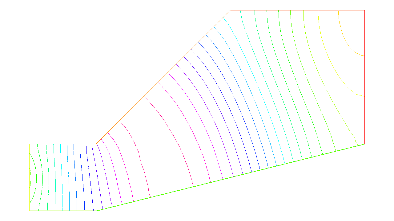
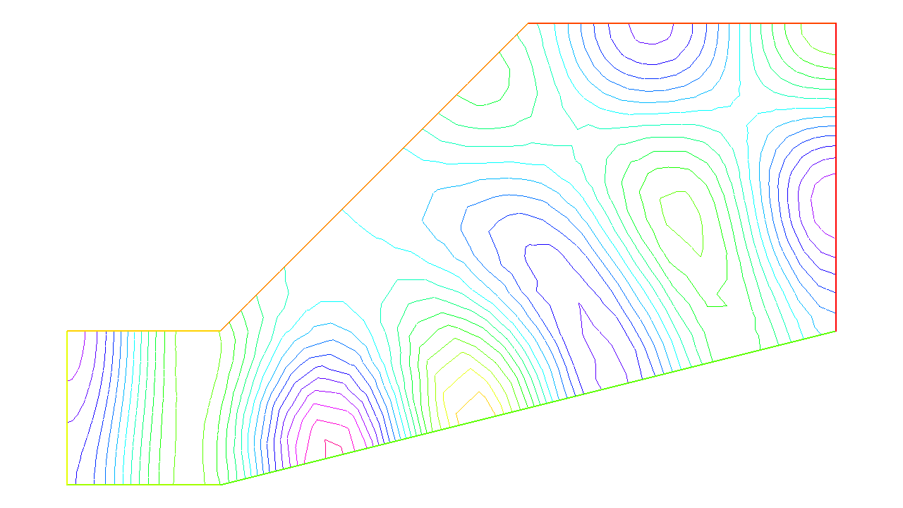
Results are on Fig. 11. But when \(kc2\) is an eigenvalue of the problem, then the solution is not unique:
if \(u_e \neq 0\) is an eigen state, then for any given solution \(u+u_e\) is another solution.
To find all the \(u_e\) one can do the following :
 1// Parameters
 2real sigma = 20; //value of the shift
 3
 4// Problem
 5// OP = A - sigma B ; // The shifted matrix
 6varf op(u1, u2)
 7   = int2d(Th)(
 8        dx(u1)*dx(u2)
 9      + dy(u1)*dy(u2)
10      - sigma* u1*u2
11   )
12   ;
13
14varf b([u1], [u2])
15   = int2d(Th)(
16        u1*u2
17   )
18   ; // No Boundary condition see note \ref{note BC EV}
19
20matrix OP = op(Vh, Vh, solver=Crout, factorize=1);
21matrix B = b(Vh, Vh, solver=CG, eps=1e-20);
22
23// Eigen values
24int nev=2; // Number of requested eigenvalues near sigma
25
26real[int] ev(nev);  // To store the nev eigenvalue
27Vh[int] eV(nev);    // To store the nev eigenvector
28
29int k=EigenValue(OP, B, sym=true, sigma=sigma, value=ev, vector=eV,
30   tol=1e-10, maxit=0, ncv=0);
31
32cout << ev(0) << " 2 eigen values " << ev(1) << endl;
33v = eV[0];
34plot(v, wait=true, ps="eigen.eps");