Static problems

Soap Film

Our starting point here will be the mathematical model to find the shape of soap film which is glued to the ring on the \(xy-\)plane:

\[C=\{(x,y);\;x=\cos t,\,y=\sin t,\,0\leq t\leq 2\pi \}\]

We assume the shape of the film is described by the graph \((x,y,u(x,y))\) of the vertical displacement \(u(x,y)\, (x^2+y^2<1)\) under a vertical pressure \(p\) in terms of force per unit area and an initial tension \(\mu\) in terms of force per unit length.

Consider the “small plane” ABCD, A:\((x,y,u(x,y))\), B:\((x,y,u(x+\delta x,y))\), C:\((x,y,u(x+\delta x,y+\delta y))\) and D:\((x,y,u(x,y+\delta y))\).

Denote by \(\vec{n}(x,y)=(n_x(x,y),n_y(x,y),n_z(x,y))\) the normal vector of the surface \(z=u(x,y)\). We see that the vertical force due to the tension \(\mu\) acting along the edge AD is \(-\mu n_x(x,y)\delta y\) and the the vertical force acting along the edge AD is:

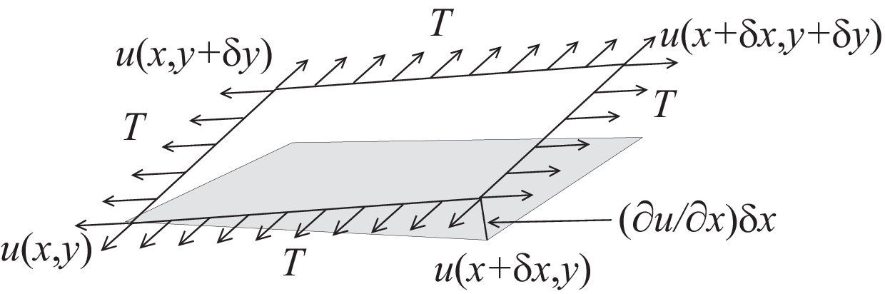
\[\mu n_x(x+\delta x,y)\delta y\simeq \mu\left(n_x(x,y)+\frac{\p n_x}{\p x}\delta x\right)(x,y)\delta y\]

Similarly, for the edges AB and DC we have:

\[-\mu n_y(x,y)\delta x,\quad\mu\left(n_y(x,y)+\p n_y/\p y\right)(x,y)\delta x\]

The force in the vertical direction on the surface ABCD due to the tension \(\mu\) is given by:

\[\mu\left(\p n_x/\p x\right)\delta x\delta y+T\left(\p n_y/\p y\right)\delta y\delta x\]

Assuming small displacements, we have:

\[\begin{split}\begin{array}{rcccl} \nu_x&=&(\p u/\p x)/\sqrt{1+(\p u/\p x)^2+(\p u/\p y)^2}&\simeq& \p u/\p x,\\ \nu_y&=&(\p u/\p y)/\sqrt{1+(\p u/\p x)^2+(\p u/\p y)^2}&\simeq& \p u/\p y \end{array}\end{split}\]

Letting \(\delta x\to dx,\, \delta y\to dy\), we have the equilibrium of the vertical displacement of soap film on ABCD by \(p\):

\[\mu dx dy\p^2 u/\p x^2 +\mu dx dy\p^2 u/\p y^2 + p dx dy = 0\]

Using the Laplace operator \(\Delta = \p^2 /\p x^2 + \p^2 /\p y^2\), we can find the virtual displacement write the following:

\[-\Delta u = f\quad \mbox{in }\Omega\]

where \(f=p/\mu\), \(\Omega =\{(x,y);\;x^{2}+y^{2}<1\}\).

Poisson’s equation appears also in electrostatics taking the form of \(f=\rho / \epsilon\) where \(\rho\) is the charge density, \(\epsilon\) the dielectric constant and \(u\) is named as electrostatic potential.

The soap film is glued to the ring \(\p \Omega =C\), then we have the boundary condition:

\[u=0\quad \mbox{on }\p \Omega\]

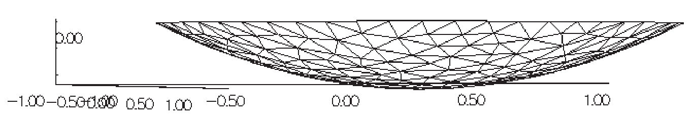
If the force is gravity, for simplify, we assume that \(f=-1\).

// Parameters
int nn = 50;
func f = -1;
func ue = (x^2+y^2-1)/4; //ue: exact solution

// Mesh
border a(t=0, 2*pi){x=cos(t); y=sin(t); label=1;}
mesh disk = buildmesh(a(nn));
plot(disk);

// Fespace
fespace femp1(disk, P1);
femp1 u, v;

// Problem
problem laplace (u, v)
    = int2d(disk)( //bilinear form
        dx(u)*dx(v)
        + dy(u)*dy(v)
    )
    - int2d(disk)( //linear form
        f*v
    )
    + on(1, u=0) //boundary condition
    ;

// Solve
laplace;

// Plot
plot (u, value=true, wait=true);

// Error
femp1 err = u - ue;
plot(err, value=true, wait=true);

cout << "error L2 = " << sqrt( int2d(disk)(err^2) )<< endl;
cout << "error H10 = " << sqrt( int2d(disk)((dx(u)-x/2)^2) + int2d(disk)((dy(u)-y/2)^2) )<< endl;

/// Re-run with a mesh adaptation ///

// Mesh adaptation
disk = adaptmesh(disk, u, err=0.01);
plot(disk, wait=true);

// Solve
laplace;
plot (u, value=true, wait=true);

// Error
err = u - ue; //become FE-function on adapted mesh
plot(err, value=true, wait=true);

cout << "error L2 = " << sqrt( int2d(disk)(err^2) )<< endl;
cout << "error H10 = " << sqrt( int2d(disk)((dx(u)-x/2)^2) + int2d(disk)((dy(u)-y/2)^2) )<< endl;

../_images/StaticProblems_SoapFilmSol.png — Fig. 136 Isovalue of \(u\)

../_images/StaticProblems_SoapFilm3D.png — Fig. 137 A side view of \(u\)

In the 37th line, the \(L^2\)-error estimation between the exact solution \(u_e\),

\[\|u_h - u_e\|_{0,\Omega}=\left(\int_{\Omega}|u_h-u_e|^2\, \d x\d y\right)^{1/2}\]

and in the following line, the \(H^1\)-error seminorm estimation:

\[|u_h - u_e|_{1,\Omega}=\left(\int_{\Omega}|\nabla u_h-\nabla u_e|^2\, \d x\d y\right)^{1/2}\]

are done on the initial mesh. The results are \(\|u_h - u_e\|_{0,\Omega}=0.000384045,\, |u_h - u_e|_{1,\Omega}=0.0375506\).

After the adaptation, we have \(\|u_h - u_e\|_{0,\Omega}=0.000109043,\, |u_h - u_e|_{1,\Omega}=0.0188411\). So the numerical solution is improved by adaptation of mesh.

Electrostatics

We assume that there is no current and a time independent charge distribution. Then the electric field \(\mathbf{E}\) satisfies:

(55)\[\begin{split}\begin{array}{rcl} \mathrm{div}\mathbf{E} &=& \rho/\epsilon\\ \mathrm{curl}\mathbf{E} &=& 0 \end{array}\end{split}\]

where \(\rho\) is the charge density and \(\epsilon\) is called the permittivity of free space.

From the equation (55) We can introduce the electrostatic potential such that \(\mathbf{E}=-\nabla \phi\). Then we have Poisson’s equation \(-\Delta \phi=f\), \(f=-\rho/\epsilon\).

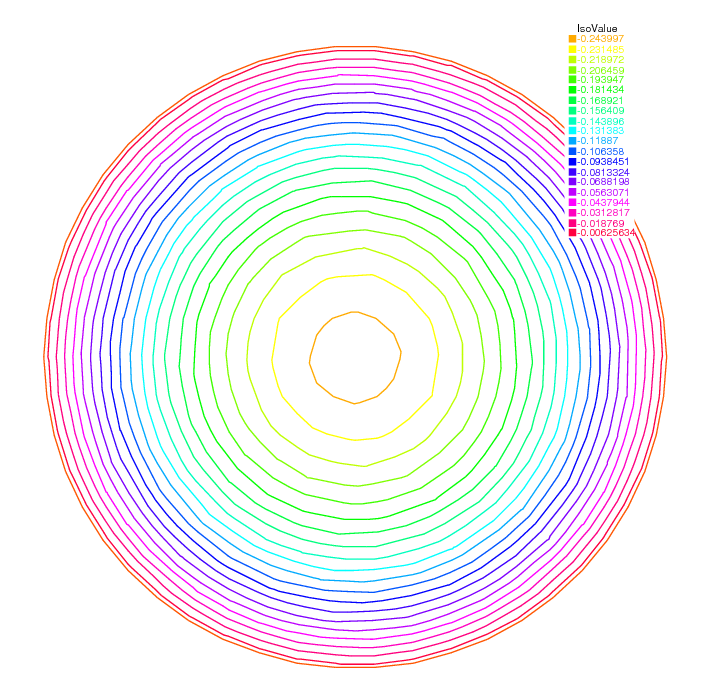
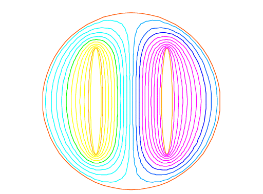
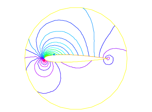
We now obtain the equipotential line which is the level curve of \(\phi\), when there are no charges except conductors \(\{C_i\}_{1,\cdots,K}\). Let us assume \(K\) conductors \(C_1,\cdots,C_K\) within an enclosure \(C_0\).

Each one is held at an electrostatic potential \(\varphi_i\). We assume that the enclosure \(C0\) is held at potential 0. In order to know \(\varphi(x)\) at any point \(x\) of the domain \(\Omega\), we must solve:

\[-\Delta \varphi =0\quad \textrm{ in }\Omega\]

where \(\Omega\) is the interior of \(C_0\) minus the conductors \(C_i\), and \(\Gamma\) is the boundary of \(\Omega\), that is \(\sum_{i=0}^N C_i\).

Here \(g\) is any function of \(x\) equal to \(\varphi_i\) on \(C_i\) and to 0 on \(C_0\). The boundary equation is a reduced form for:

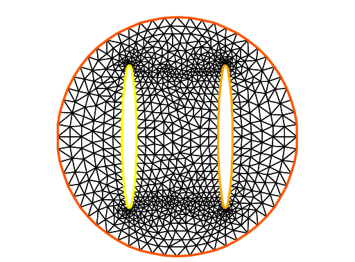
\[\varphi =\varphi_{i}\;\text{on }C_{i},\;i=1...N,\varphi =0\;\text{on }C_{0}.\]

First we give the geometrical informations; \(C_0=\{(x,y);\; x^2+y^2=5^2\}\), \(C_1=\{(x,y):\;\frac{1}{0.3^2}(x-2)^2+\frac{1}{3^2}y^2=1\}\), \(C_2=\{(x,y):\; \frac{1}{0.3^2}(x+2)^2+\frac{1}{3^2}y^2=1\}\).

Let \(\Omega\) be the disk enclosed by \(C_0\) with the elliptical holes enclosed by \(C_1\) and \(C_2\). Note that \(C_0\) is described counterclockwise, whereas the elliptical holes are described clockwise, because the boundary must be oriented so that the computational domain is to its left.

// Mesh
border C0(t=0, 2*pi){x=5*cos(t); y=5*sin(t);}
border C1(t=0, 2*pi){x=2+0.3*cos(t); y=3*sin(t);}
border C2(t=0, 2*pi){x=-2+0.3*cos(t); y=3*sin(t);}

mesh Th = buildmesh(C0(60) + C1(-50) + C2(-50));
plot(Th);

// Fespace
fespace Vh(Th, P1);
Vh uh, vh;

// Problem
problem Electro (uh, vh)
    = int2d(Th)( //bilinear
        dx(uh)*dx(vh)
        + dy(uh)*dy(vh)
    )
    + on(C0, uh=0) //boundary condition on C_0
    + on(C1, uh=1) //+1 volt on C_1
    + on(C2, uh=-1) //-1 volt on C_2
    ;

// Solve
Electro;
plot(uh);

../_images/StaticProblems_ElectrostaticsMesh.png — Fig. 138 Disk with two elliptical holes

../_images/StaticProblems_Electrostatics.png — Fig. 139 Equipotential lines where \(C_1\) is located in right hand side

Aerodynamics

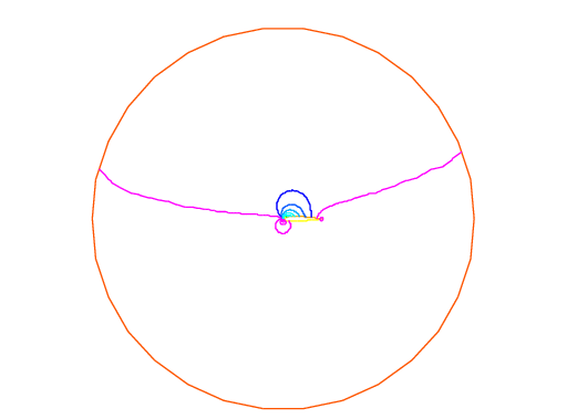
Let us consider a wing profile \(S\) in a uniform flow. Infinity will be represented by a large circle \(\Gamma_{\infty}\). As previously, we must solve:

(56)\[\Delta \varphi=0\quad\textrm{in }\Omega, \quad \varphi|_S=c,\quad \varphi|_{\Gamma_{\infty}}=u_{\infty 1x}-u_{\infty2x}\]

where \(\Omega\) is the area occupied by the fluid, \(u_{\infty}\) is the air speed at infinity, \(c\) is a constant to be determined so that \(\p_n\varphi\) is continuous at the trailing edge \(P\) of \(S\) (so-called Kutta-Joukowski condition). Lift is proportional to \(c\).

To find \(c\) we use a superposition method. As all equations in (56) are linear, the solution \(\varphi_c\) is a linear function of \(c\)

\[\varphi_c = \varphi_0 + c\varphi_1\]

where \(\varphi_0\) is a solution of (56) with \(c = 0\) and \(\varphi_1\) is a solution with \(c = 1\) and zero speed at infinity.

With these two fields computed, we shall determine \(c\) by requiring the continuity of \(\p \varphi /\p n\) at the trailing edge. An equation for the upper surface of a NACA0012 (this is a classical wing profile in aerodynamics; the rear of the wing is called the trailing edge) is:

\[y = 0.17735\sqrt{x} - 0.075597x - 0.212836x^2 + 0.17363x^3 - 0.06254x^4\]

Taking an incidence angle \(\alpha\) such that \(\tan \alpha = 0.1\), we must solve:

\[-\Delta\varphi = 0\qquad \textrm{in }\Omega, \quad \varphi|_{\Gamma_1} = y - 0.1x,\quad \varphi |_{\Gamma_2} = c\]

where \(\Gamma_2\) is the wing profile and \(\Gamma_1\) is an approximation of infinity. One finds \(c\) by solving:

\[\begin{split}\begin{array}{ccccccc} -\Delta\varphi_0 &= 0 &\textrm{in }\Omega&,\qquad \varphi_0|_{\Gamma_1} &= y - 0.1x&, \quad \varphi_0|_{\Gamma_2} &= 0,\\ -\Delta\varphi_1 &= 0 &\textrm{in }\Omega&, \qquad \varphi_1|_{\Gamma_1} &= 0&, \quad \varphi_1|_{\Gamma_2} &= 1 \end{array}\end{split}\]

The solution \(\varphi = \varphi_0+c\varphi_1\) allows us to find \(c\) by writing that \(\p_n\varphi\) has no jump at the trailing edge \(P = (1, 0)\).

We have \(\p n\varphi -(\varphi (P^+)-\varphi (P))/\delta\) where \(P^+\) is the point just above \(P\) in the direction normal to the profile at a distance \(\delta\). Thus the jump of \(\p_n\varphi\) is \((\varphi_0|_{P^+} +c(\varphi_1|_{P^+} -1))+(\varphi_0|_{P^-} +c(\varphi_1|_{P^-} -1))\) divided by \(\delta\) because the normal changes sign between the lower and upper surfaces. Thus

\[c = -\frac{\varphi_0|_{P^+} + \varphi_0|_{P^-}} {(\varphi_1|_{P^+} + \varphi_1|_{P^-} - 2)} ,\]

which can be programmed as:

\[c = -\frac{\varphi_0(0.99, 0.01) + \varphi_0(0.99,-0.01)} {(\varphi_1(0.99, 0.01) + \varphi_1(0.99,-0.01) - 2)} .\]

// Mesh
border a(t=0, 2*pi){x=5*cos(t); y=5*sin(t);}
border upper(t=0, 1) {
    x=t;
    y=0.17735*sqrt(t)-0.075597*t - 0.212836*(t^2) + 0.17363*(t^3) - 0.06254*(t^4);
}
border lower(t=1, 0) {
    x=t;
    y=-(0.17735*sqrt(t) - 0.075597*t - 0.212836*(t^2) + 0.17363*(t^3) - 0.06254*(t^4));
}
border c(t=0, 2*pi){x=0.8*cos(t)+0.5; y=0.8*sin(t);}

mesh Zoom = buildmesh(c(30) + upper(35) + lower(35));
mesh Th = buildmesh(a(30) + upper(35) + lower(35));

// Fespace
fespace Vh(Th, P2);
Vh psi0, psi1, vh;

fespace ZVh(Zoom, P2);

// Problem
solve Joukowski0(psi0, vh)
    = int2d(Th)(
        dx(psi0)*dx(vh)
        + dy(psi0)*dy(vh)
    )
    + on(a, psi0=y-0.1*x)
    + on(upper, lower, psi0=0)
    ;

plot(psi0);

solve Joukowski1(psi1,vh)
    = int2d(Th)(
        dx(psi1)*dx(vh)
        + dy(psi1)*dy(vh)
    )
    + on(a, psi1=0)
    + on(upper, lower, psi1=1);

plot(psi1);

//continuity of pressure at trailing edge
real beta = psi0(0.99,0.01) + psi0(0.99,-0.01);
beta = -beta / (psi1(0.99,0.01) + psi1(0.99,-0.01)-2);

Vh psi = beta*psi1 + psi0;
plot(psi);

ZVh Zpsi = psi;
plot(Zpsi, bw=true);

ZVh cp = -dx(psi)^2 - dy(psi)^2;
plot(cp);

ZVh Zcp = cp;
plot(Zcp, nbiso=40);

../_images/StaticProblems_Aerodynamics1.png — Fig. 140 Isovalue of \(cp = -(\p_x\psi)^2 - (\p_y\psi)^2\)

../_images/StaticProblems_Aerodynamics2.png — Fig. 141 Zooming of \(cp\)

Error estimation

There are famous estimation between the numerical result \(u_h\) and the exact solution \(u\) of the Poisson’s problem:

If triangulations \(\{\mathcal{T}_h\}_{h\downarrow 0}\) is regular (see Regular Triangulation), then we have the estimates:

(57)\[\begin{split}\begin{array}{rcl} |\nabla u - \nabla u_h|_{0,\Omega} &\le& C_1h \\ \|u - u_h\|_{0,\Omega} &\le& C_2h^2 \end{array}\end{split}\]

with constants \(C_1,\, C_2\) independent of \(h\), if \(u\) is in \(H^2(\Omega)\). It is known that \(u\in H^2(\Omega)\) if \(\Omega\) is convex.

In this section we check (57). We will pick up numericall error if we use the numerical derivative, so we will use the following for (57).

\[\begin{split}\begin{array}{rcl} \int_{\Omega}|\nabla u - \nabla u_h|^2\, \d x\d y &=&\int_{\Omega}\nabla u\cdot \nabla(u - 2u_h)\, \d x\d y+ \int_{\Omega}\nabla u_h\cdot \nabla u_h\, \d x\d y\\ &=&\int_{\Omega}f(u-2u_h)\, \d x\d y+\int_{\Omega}fu_h\, \d x\d y \end{array}\end{split}\]

The constants \(C_1,\, C_2\) are depend on \(\mathcal{T}_h\) and \(f\), so we will find them by FreeFEM.

In general, we cannot get the solution \(u\) as a elementary functions even if spetical functions are added. Instead of the exact solution, here we use the approximate solution \(u_0\) in \(V_h(\mathcal{T}_h,P_2),\, h\sim 0\).

// Parameters
func f = x*y;

//Mesh
mesh Th0 = square(100, 100);

// Fespace
fespace V0h(Th0, P2);
V0h u0, v0;

// Problem
solve Poisson0 (u0, v0)
    = int2d(Th0)(
        dx(u0)*dx(v0)
        + dy(u0)*dy(v0)
    )
    - int2d(Th0)(
        f*v0
    )
    + on(1, 2, 3, 4, u0=0)
    ;
plot(u0);

// Error loop
real[int] errL2(10), errH1(10);
for (int i = 1; i <= 10; i++){
    // Mesh
    mesh Th = square(5+i*3,5+i*3);

    // Fespace
    fespace Vh(Th, P1);
    Vh u, v;
    fespace Ph(Th, P0);
    Ph h = hTriangle; //get the size of all triangles

    // Problem
    solve Poisson (u, v)
        = int2d(Th)(
            dx(u)*dx(v)
            + dy(u)*dy(v)
        )
        - int2d(Th)(
            f*v
        )
        + on(1, 2, 3, 4, u=0)
        ;

    // Error
    V0h uu = u; //interpolate solution on first mesh
    errL2[i-1] = sqrt( int2d(Th0)((uu - u0)^2) )/h[].max^2;
    errH1[i-1] = sqrt( int2d(Th0)(f*(u0 - 2*uu + uu)) )/h[].max;
}

// Display
cout << "C1 = " << errL2.max << "("<<errL2.min<<")" << endl;
cout << "C2 = " << errH1.max << "("<<errH1.min<<")" << endl;

We can guess that \(C_1=0.0179253(0.0173266)\) and \(C_2=0.0729566(0.0707543)\), where the numbers inside the parentheses are minimum in calculation.

Periodic Boundary Conditions

We now solve the Poisson equation:

\[-\Delta u = sin(x+\pi/4.)*cos(y+\pi/4.)\]

on the square \(]0,2\pi[^2\) under bi-periodic boundary condition \(u(0,y)=u(2\pi,y)\) for all \(y\) and \(u(x,0)=u(x,2\pi)\) for all \(x\).

These boundary conditions are achieved from the definition of the periodic finite element space.

// Parameters
func f = sin(x+pi/4.)*cos(y+pi/4.); //right hand side

// Mesh
mesh Th = square(10, 10, [2*x*pi, 2*y*pi]);

// Fespace
//defined the fespace with periodic condition
//label: 2 and 4 are left and right side with y the curve abscissa
//       1 and 2 are bottom and upper side with x the curve abscissa
fespace Vh(Th, P2, periodic=[[2, y], [4, y], [1, x], [3, x]]);
Vh uh, vh;

// Problem
problem laplace (uh, vh)
    = int2d(Th)(
        uh*vh*1.0e-10 // to fix the constant
        + dx(uh)*dx(vh)
        + dy(uh)*dy(vh)
    )
    + int2d(Th)(
        - f*vh
    )
    ;

// Solve
laplace;

// Plot
plot(uh, value=true);

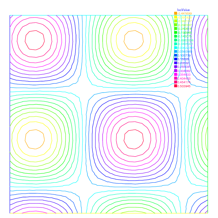
../_images/StaticProblems_PeriodicBoundaryConditions.png — Fig. 142 The isovalue of solution \(u\) with periodic boundary condition

The periodic condition does not necessarily require parallel boundaries. The following example give such example.

Tip

Periodic boundary conditions - non-parallel boundaries

// Parameters
int n = 10;
real r = 0.25;
real r2 = 1.732;
func f = (y+x+1)*(y+x-1)*(y-x+1)*(y-x-1);

// Mesh
border a(t=0, 1){x=-t+1; y=t; label=1;};
border b(t=0, 1){x=-t; y=1-t; label=2;};
border c(t=0, 1){x=t-1; y=-t; label=3;};
border d(t=0, 1){x=t; y=-1+t; label=4;};
border e(t=0, 2*pi){x=r*cos(t); y=-r*sin(t); label=0;};
mesh Th = buildmesh(a(n) + b(n) + c(n) + d(n) + e(n));
plot(Th, wait=true);

// Fespace
//warning for periodic condition:
//side a and c
//on side a (label 1) $ x \in [0,1] $ or $ x-y\in [-1,1] $
//on side c (label 3) $ x \in [-1,0]$ or $ x-y\in[-1,1] $
//so the common abscissa can be respectively $x$ and $x+1$
//or you can can try curviline abscissa $x-y$ and $x-y$
//1 first way
//fespace Vh(Th, P2, periodic=[[2, 1+x], [4, x], [1, x], [3, 1+x]]);
//2 second way
fespace Vh(Th, P2, periodic=[[2, x+y], [4, x+y], [1, x-y], [3, x-y]]);
Vh uh, vh;

// Problem
real intf = int2d(Th)(f);
real mTh = int2d(Th)(1);
real k =  intf / mTh;
problem laplace (uh, vh)
    = int2d(Th)(
        uh*vh*1.0e-10 // to fix the constant
        + dx(uh)*dx(vh)
        + dy(uh)*dy(vh)
    )
    + int2d(Th)(
        (k-f)*vh
    )
    ;

// Solve
laplace;

// Plot
plot(uh, wait=true);

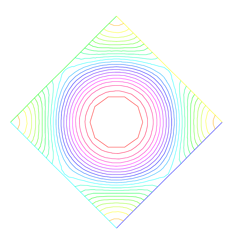
../_images/StaticProblems_PeriodicBoundaryConditions2.png — Fig. 143 The isovalue of solution \(u\) for \(\Delta u = ((y+x)^{2}+1)((y-x)^{2}+1) - k\), in \(\Omega\) and \(\p_{n} u =0\) on hole, and with two periodic boundary condition on external border

An other example with no equal border, just to see if the code works.

Tip

Periodic boundary conditions - non-equal border

// Macro
//irregular boundary condition to build border AB
macro LINEBORDER(A, B, lab)
    border A#B(t=0,1){ real t1=1.-t;
    x=A#x*t1+B#x*t;
    y=A#y*t1+B#y*t;
    label=lab; } //EOM
// compute \||AB|\| A=(ax,ay) et B =(bx,by)
macro dist(ax, ay, bx, by)
    sqrt(square((ax)-(bx)) + square((ay)-(by))) //EOM
macro Grad(u) [dx(u), dy(u)] //EOM

// Parameters
int n = 10;
real Ax = 0.9, Ay = 1;
real Bx = 2, By = 1;
real Cx = 2.5, Cy = 2.5;
real Dx = 1, Dy = 2;
real gx = (Ax+Bx+Cx+Dx)/4.;
real gy = (Ay+By+Cy+Dy)/4.;

// Mesh
LINEBORDER(A,B,1)
LINEBORDER(B,C,2)
LINEBORDER(C,D,3)
LINEBORDER(D,A,4)
mesh Th=buildmesh(AB(n)+BC(n)+CD(n)+DA(n),fixedborder=1);

// Fespace
real l1 = dist(Ax,Ay,Bx,By);
real l2 = dist(Bx,By,Cx,Cy);
real l3 = dist(Cx,Cy,Dx,Dy);
real l4 = dist(Dx,Dy,Ax,Ay);
func s1 = dist(Ax,Ay,x,y)/l1; //absisse on AB = ||AX||/||AB||
func s2 = dist(Bx,By,x,y)/l2; //absisse on BC = ||BX||/||BC||
func s3 = dist(Cx,Cy,x,y)/l3; //absisse on CD = ||CX||/||CD||
func s4 = dist(Dx,Dy,x,y)/l4; //absisse on DA = ||DX||/||DA||
verbosity = 6; //to see the abscisse value of the periodic condition
fespace Vh(Th, P1, periodic=[[1, s1], [3, s3], [2, s2], [4, s4]]);
verbosity = 1; //reset verbosity
Vh u, v;

real cc = 0;
cc = int2d(Th)((x-gx)*(y-gy)-cc)/Th.area;
cout << "compatibility = " << int2d(Th)((x-gx)*(y-gy)-cc) <<endl;

// Problem
solve Poisson (u, v)
    = int2d(Th)(
        Grad(u)'*Grad(v)
        + 1e-10*u*v
    )
    -int2d(Th)(
        10*v*((x-gx)*(y-gy)-cc)
    )
    ;

// Plot
plot(u, value=true);

Tip

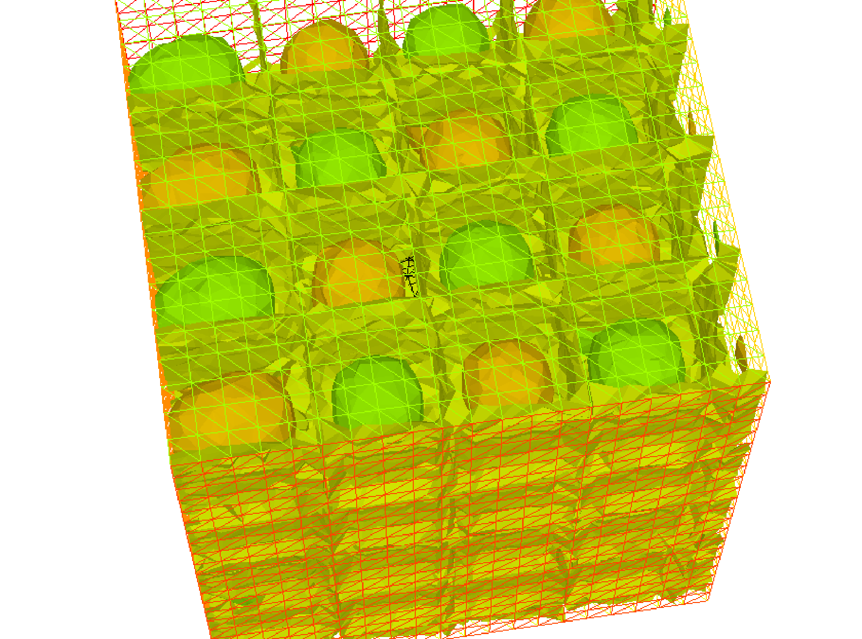
Periodic boundry conditions - Poisson cube-balloon

load "msh3" load "tetgen" load "medit"

// Parameters
real hs = 0.1; //mesh size on sphere
int[int] N = [20, 20, 20];
real [int,int] B = [[-1, 1], [-1, 1], [-1, 1]];
int [int,int] L = [[1, 2], [3, 4], [5, 6]];

real x0 = 0.3, y0 = 0.4, z0 = 06;
func f = sin(x*2*pi+x0)*sin(y*2*pi+y0)*sin(z*2*pi+z0);

// Mesh
bool buildTh = 0;
mesh3 Th;
try { //a way to build one time the mesh or read it if the file exist
    Th = readmesh3("Th-hex-sph.mesh");
}
catch (...){
    buildTh = 1;
}

if (buildTh){
    include "MeshSurface.idp"

    // Surface Mesh
    mesh3 ThH = SurfaceHex(N, B, L, 1);
    mesh3 ThS = Sphere(0.5, hs, 7, 1);

    mesh3 ThHS = ThH + ThS;

    real voltet = (hs^3)/6.;
    real[int] domain = [0, 0, 0, 1, voltet, 0, 0, 0.7, 2, voltet];
    Th = tetg(ThHS, switch="pqaAAYYQ", nbofregions=2, regionlist=domain);

    savemesh(Th, "Th-hex-sph.mesh");
}

// Fespace
fespace Ph(Th, P0);
Ph reg = region;
cout << " centre = " << reg(0,0,0) << endl;
cout << " exterieur = " << reg(0,0,0.7) << endl;

verbosity = 50;
fespace Vh(Th, P1, periodic=[[3, x, z], [4, x, z], [1, y, z], [2, y, z], [5, x, y], [6, x, y]]);
verbosity = 1;
Vh uh,vh;

// Macro
macro Grad(u) [dx(u),dy(u),dz(u)] // EOM

// Problem
problem Poisson (uh, vh)
    = int3d(Th, 1)(
        Grad(uh)'*Grad(vh)*100
    )
    + int3d(Th, 2)(
        Grad(uh)'*Grad(vh)*2
    )
    + int3d(Th)(
        vh*f
    )
    ;

// Solve
Poisson;

// Plot
plot(uh, wait=true, nbiso=6);
medit("uh", Th, uh);

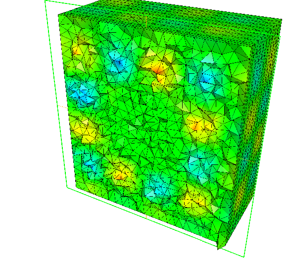
../_images/StaticProblems_PeriodicBoundaryConditionsPoisson1.png — Fig. 144 View of the surface isovalue of periodic solution \(uh\)

../_images/StaticProblems_PeriodicBoundaryConditionsPoisson2.png — Fig. 145 View a the cut of the solution \(uh\) with ffmedit

Poisson Problems with mixed boundary condition

Here we consider the Poisson equation with mixed boundary conditions:

For given functions \(f\) and \(g\), find \(u\) such that:

\[\begin{split}\begin{array}{rcll} -\Delta u &=& f & \textrm{ in }\Omega\\ u &=& g &\textrm{ on }\Gamma_D\\ \p u/\p n &=& 0 &\textrm{ on }\Gamma_N \end{array}\end{split}\]

where \(\Gamma_D\) is a part of the boundary \(\Gamma\) and \(\Gamma_N=\Gamma\setminus \overline{\Gamma_D}\).

The solution \(u\) has the singularity at the points \(\{\gamma_1,\gamma_2\}=\overline{\Gamma_D}\cap\overline{\Gamma_N}\).

When \(\Omega=\{(x,y);\; -1<x<1,\, 0<y<1\}\), \(\Gamma_N=\{(x,y);\; -1\le x<0,\, y=0\}\), \(\Gamma_D=\p \Omega\setminus \Gamma_N\), the singularity will appear at \(\gamma_1=(0,0),\, \gamma_2(-1,0)\), and \(u\) has the expression:

\[u=K_iu_S + u_R,\, u_R\in H^2(\textrm{near }\gamma_i),\, i=1,2\]

with a constants \(K_i\).

Here \(u_S = r_j^{1/2}\sin(\theta_j/2)\) by the local polar coordinate \((r_j,\theta_j\) at \(\gamma_j\) such that \((r_1,\theta_1)=(r,\theta)\).

Instead of polar coordinate system \((r,\theta)\), we use that \(r\) = sqrt (\(x^2+y^2\)) and \(\theta\) = atan2 (\(y,x\)) in FreeFEM.

Assume that \(f=-2\times 30(x^2+y^2)\) and \(g=u_e=10(x^2+y^2)^{1/4}\sin\left([\tan^{-1}(y/x)]/2\right)+30(x^2y^2)\), where \(u_e\)S is the exact solution.

// Parameters
func f = -2*30*(x^2+y^2); //given function
//the singular term of the solution is K*us (K: constant)
func us = sin(atan2(y,x)/2)*sqrt( sqrt(x^2+y^2) );
real K = 10.;
func ue = K*us + 30*(x^2*y^2);

// Mesh
border N(t=0, 1){x=-1+t; y=0; label=1;};
border D1(t=0, 1){x=t; y=0; label=2;};
border D2(t=0, 1){x=1; y=t; label=2;};
border D3(t=0, 2){x=1-t; y=1; label=2;};
border D4(t=0, 1){x=-1; y=1-t; label=2;};

mesh T0h = buildmesh(N(10) + D1(10) + D2(10) + D3(20) + D4(10));
plot(T0h, wait=true);

// Fespace
fespace V0h(T0h, P1);
V0h u0, v0;

//Problem
solve Poisson0 (u0, v0)
    = int2d(T0h)(
        dx(u0)*dx(v0)
        + dy(u0)*dy(v0)
    )
    - int2d(T0h)(
        f*v0
    )
    + on(2, u0=ue)
    ;

// Mesh adaptation by the singular term
mesh Th = adaptmesh(T0h, us);
for (int i = 0; i < 5; i++)
mesh Th = adaptmesh(Th, us);

// Fespace
fespace Vh(Th, P1);
Vh u, v;

// Problem
solve Poisson (u, v)
    = int2d(Th)(
        dx(u)*dx(v)
        + dy(u)*dy(v)
    )
    - int2d(Th)(
        f*v
    )
    + on(2, u=ue)
    ;

// Plot
plot(Th);
plot(u, wait=true);

// Error in H1 norm
Vh uue = ue;
real H1e = sqrt( int2d(Th)(dx(uue)^2 + dy(uue)^2 + uue^2) );
Vh err0 = u0 - ue;
Vh err = u - ue;
Vh H1err0 = int2d(Th)(dx(err0)^2 + dy(err0)^2 + err0^2);
Vh H1err = int2d(Th)(dx(err)^2 + dy(err)^2 + err^2);
cout << "Relative error in first mesh = "<< int2d(Th)(H1err0)/H1e << endl;
cout << "Relative error in adaptive mesh = "<< int2d(Th)(H1err)/H1e << endl;

From line 35 to 37, mesh adaptations are done using the base of singular term.

In line 61, H1e = \(|u_e|_{1,\Omega}\) is calculated.

In lines 64 and 65, the relative errors are calculated, that is:

\[\begin{split}\begin{array}{rcl} \|u^0_h-u_e\|_{1,\Omega}/H1e&=&0.120421\\ \|u^a_h-u_e\|_{1,\Omega}/H1e&=&0.0150581 \end{array}\end{split}\]

where \(u^0_h\) is the numerical solution in T0h and \(u^a_h\) is u in this program.

Poisson with mixed finite element

Here we consider the Poisson equation with mixed boundary value problems:

For given functions \(f\) , \(g_d\), \(g_n\), find \(p\) such that

\[\begin{split}\begin{array}{rcll} -\Delta p &=& 1 & \textrm{ in }\Omega\\ p &=& g_d & \textrm{ on }\Gamma_D\\ \p p/\p n &=& g_n & \textrm{ on }\Gamma_N \end{array}\end{split}\]

where \(\Gamma_D\) is a part of the boundary \(\Gamma\) and \(\Gamma_N=\Gamma\setminus \overline{\Gamma_D}\).

The mixed formulation is: find \(p\) and \(\mathbf{u}\) such that:

\[\begin{split}\begin{array}{rcll} \nabla p + \mathbf{u} &=& \mathbf{0} & \textrm{ in }\Omega\\ \nabla. \mathbf{u} &=& f & \textrm{ in }\Omega\\ p &=& g_d & \textrm{ on }\Gamma_D\\ \p u. n &=& \mathbf{g}_n.n & \textrm{ on }\Gamma_N \end{array}\end{split}\]

where \(\mathbf{g}_n\) is a vector such that \(\mathbf{g}_n.n = g_n\).

The variational formulation is:

\[\begin{split}\begin{array}{rcl} \forall \mathbf{v} \in \mathbb{V}_0: & \int_\Omega p \nabla.v + \mathbf{v} \mathbf{v} &= \int_{\Gamma_d} g_d \mathbf{v}.n\\ \forall {q} \in \mathbb{P}: & \int_\Omega q \nabla.u &= \int_\Omega q f\nonumber\\ & \p u. n &= \mathbf{g}_n.n \quad \textrm{on }\Gamma_N \end{array}\end{split}\]

where the functional space are:

\[\mathbb{P}= L^2(\Omega), \qquad\mathbb{V}= H(div)=\{\mathbf{v}\in L^2(\Omega)^2,\nabla.\mathbf{v}\in L^2(\Omega)\}\]

and:

\[\mathbb{V}_0 = \{\mathbf{v}\in \mathbb{V};\quad\mathbf{v}. n = 0 \quad\mathrm{on }\;\;\Gamma_N\}\]

To write the FreeFEM example, we have just to choose the finites elements spaces.

Here \(\mathbb{V}\) space is discretize with Raviart-Thomas finite element RT0 and \(\mathbb{P}\) is discretize by constant finite element P0.

Example 9.10 LaplaceRT.edp

// Parameters
func gd = 1.;
func g1n = 1.;
func g2n = 1.;

// Mesh
mesh Th = square(10, 10);

// Fespace
fespace Vh(Th, RT0);
Vh [u1, u2];
Vh [v1, v2];

fespace Ph(Th, P0);
Ph p, q;

// Problem
problem laplaceMixte ([u1, u2, p], [v1, v2, q], solver=GMRES, eps=1.0e-10, tgv=1e30, dimKrylov=150)
    = int2d(Th)(
        p*q*1e-15 //this term is here to be sure
        // that all sub matrix are inversible (LU requirement)
        + u1*v1
        + u2*v2
        + p*(dx(v1)+dy(v2))
        + (dx(u1)+dy(u2))*q
    )
    + int2d(Th) (
        q
    )
    - int1d(Th, 1, 2, 3)(
        gd*(v1*N.x +v2*N.y)
    )
    + on(4, u1=g1n, u2=g2n)
    ;

// Solve
laplaceMixte;

// Plot
plot([u1, u2], coef=0.1, wait=true, value=true);
plot(p, fill=1, wait=true, value=true);

Metric Adaptation and residual error indicator

We do metric mesh adaption and compute the classical residual error indicator \(\eta_{T}\) on the element \(T\) for the Poisson problem.

First, we solve the same problem as in a previous example.

// Parameters
real[int] viso(21);
for (int i = 0; i < viso.n; i++)
viso[i] = 10.^(+(i-16.)/2.);
real error = 0.01;
func f = (x-y);

// Mesh
border ba(t=0, 1.0){x=t; y=0; label=1;}
border bb(t=0, 0.5){x=1; y=t; label=2;}
border bc(t=0, 0.5){x=1-t; y=0.5; label=3;}
border bd(t=0.5, 1){x=0.5; y=t; label=4;}
border be(t=0.5, 1){x=1-t; y=1; label=5;}
border bf(t=0.0, 1){x=0; y=1-t; label=6;}
mesh Th = buildmesh(ba(6) + bb(4) + bc(4) + bd(4) + be(4) + bf(6));

// Fespace
fespace Vh(Th, P2);
Vh u, v;

fespace Nh(Th, P0);
Nh rho;

// Problem
problem Problem1 (u, v, solver=CG, eps=1.0e-6)
    = int2d(Th, qforder=5)(
        u*v*1.0e-10
        + dx(u)*dx(v)
        + dy(u)*dy(v)
    )
    + int2d(Th, qforder=5)(
        - f*v
    )
    ;

Now, the local error indicator \(\eta_{T}\) is:

\[\eta_{T} =\left( h_{T}^{2} || f + \Delta u_{{h}} ||_{L^{2}(T)}^{2} +\sum_{e\in \mathcal{E}_{K}} h_{e} \,||\, [ \frac{\p u_{h}}{\p n_{k}}] \,||^{2}_{L^{2}(e)} \right)^{\frac{1}{2}}\]

where \(h_{T}\) is the longest edge of \(T\), \({\cal E}_T\) is the set of \(T\) edge not on \(\Gamma=\p \Omega\), \(n_{T}\) is the outside unit normal to \(K\), \(h_{e}\) is the length of edge \(e\), \([ g ]\) is the jump of the function \(g\) across edge (left value minus right value).

Of course, we can use a variational form to compute \(\eta_{T}^{2}\), with test function constant function in each triangle.

// Error
varf indicator2 (uu, chiK)
    = intalledges(Th)(
        chiK*lenEdge*square(jump(N.x*dx(u) + N.y*dy(u)))
    )
    + int2d(Th)(
        chiK*square(hTriangle*(f + dxx(u) + dyy(u)))
    )
    ;

// Mesh adaptation loop
for (int i = 0; i < 4; i++){
    // Solve
    Problem1;
    cout << u[].min << " " << u[].max << endl;
    plot(u, wait=true);

    // Error
    rho[] = indicator2(0, Nh);
    rho = sqrt(rho);
    cout << "rho = min " << rho[].min << " max=" << rho[].max << endl;
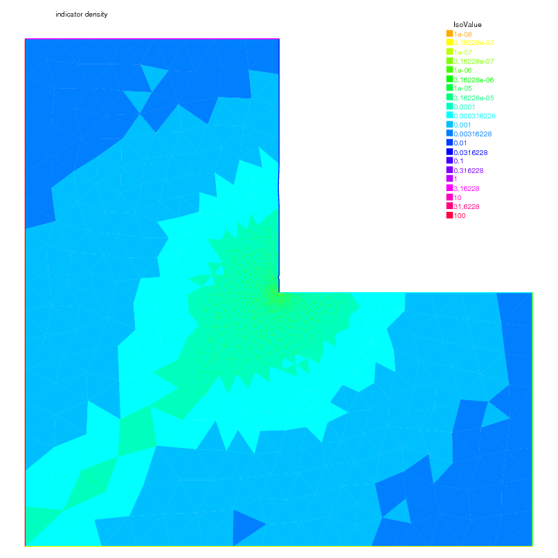
    plot(rho, fill=true, wait=true, cmm="indicator density", value=true, viso=viso, nbiso=viso.n);

    // Mesh adaptation
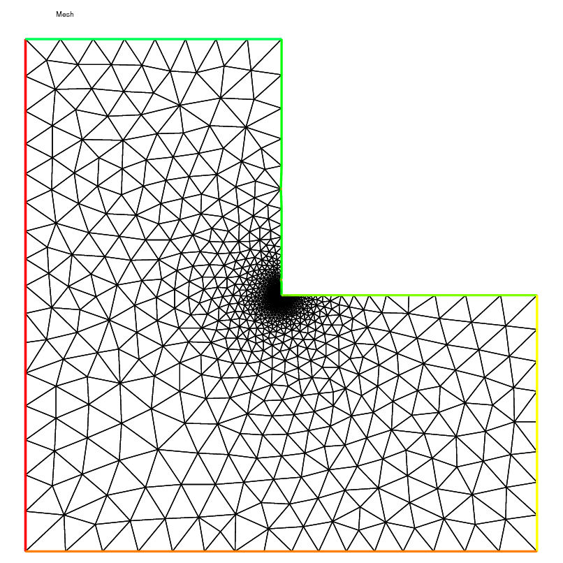
    plot(Th, wait=true, cmm="Mesh (before adaptation)");
    Th = adaptmesh(Th, [dx(u), dy(u)], err=error, anisomax=1);
    plot(Th, wait=true, cmm="Mesh (after adaptation)");
    u = u;
    rho = rho;
    error = error/2;
}

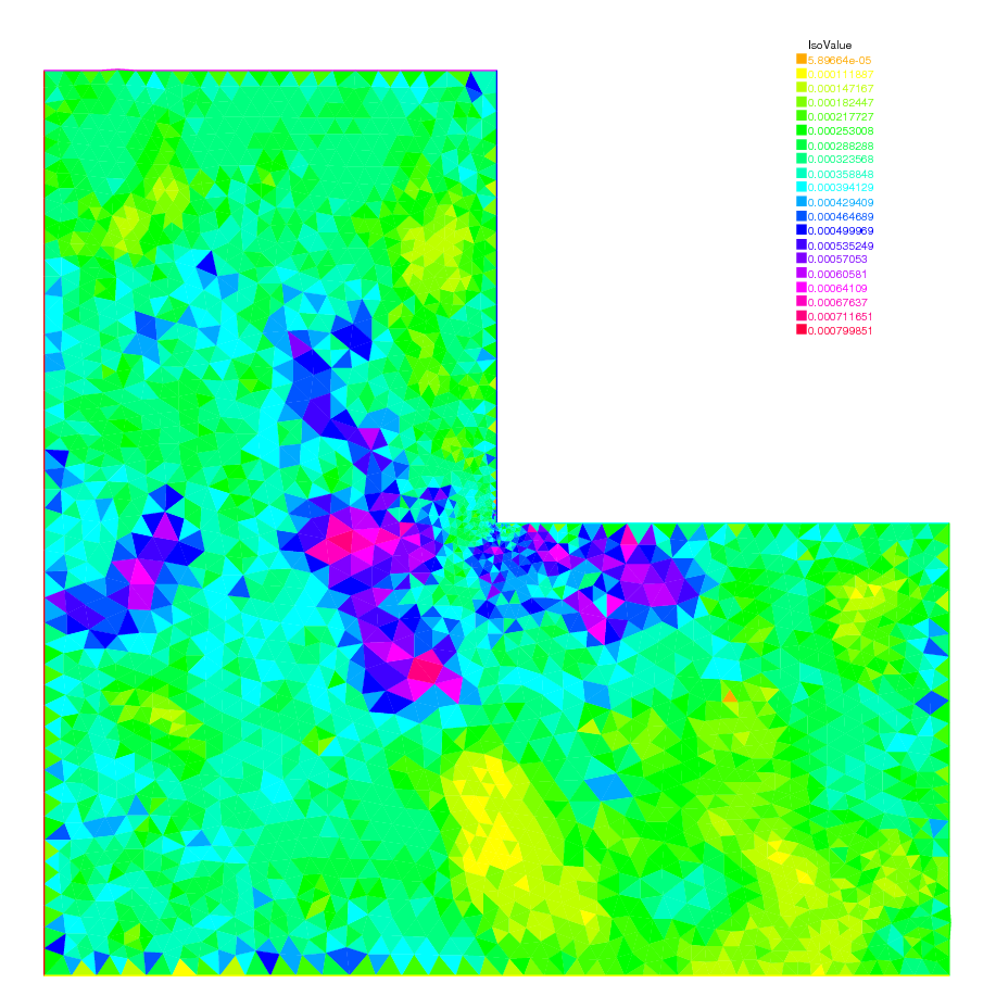
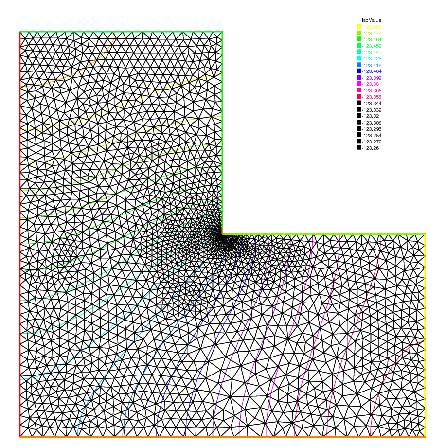
If the method is correct, we expect to look the graphics by an almost constant function \(\eta\) on your computer as in Fig. 146 and Fig. 147.

../_images/StaticProblems_MetricAdaptation.png — Fig. 146 Density of the error indicator with isotropic \(P_{2}\) metric

../_images/StaticProblems_MetricAdaptation2.png — Fig. 147 Density of the error indicator with isotropic \(P_{2}\) metric

Adaptation using residual error indicator

In the previous example we compute the error indicator, now we use it, to adapt the mesh. The new mesh size is given by the following formulae:

\[h_{n+1}(x) = \frac{h_{n}(x)}{f_{n}(\eta_K(x))}\]

where \(\eta_n(x)\) is the level of error at point \(x\) given by the local error indicator, \(h_n\) is the previous “mesh size” field, and \(f_n\) is a user function define by \(f_n = min(3,max(1/3,\eta_n / \eta_n^* ))\) where \(\eta_n^* = mean(\eta_n) c\), and \(c\) is an user coefficient generally close to one.

First a macro MeshSizecomputation is defined to get a \(P_1\) mesh size as the average of edge length.

// macro the get the current mesh size parameter
// in:
// Th the mesh
// Vh P1 fespace on Th
// out :
// h: the Vh finite element finite set to the current mesh size
macro MeshSizecomputation (Th, Vh, h)
{
    real[int] count(Th.nv);
    /*mesh size (lenEdge = integral(e) 1 ds)*/
    varf vmeshsizen (u, v) = intalledges(Th, qfnbpE=1)(v);
    /*number of edges per vertex*/
    varf vedgecount (u, v) = intalledges(Th, qfnbpE=1)(v/lenEdge);
    /*mesh size*/
    count = vedgecount(0, Vh);
    h[] = 0.;
    h[] = vmeshsizen(0, Vh);
    cout << "count min = " << count.min << " max = " << count.max << endl;
    h[] = h[]./count;
    cout << "-- bound meshsize = " << h[].min << " " << h[].max << endl;
} //

A second macro to re-mesh according to the new mesh size.

// macro to remesh according the de residual indicator
// in:
// Th the mesh
// Ph P0 fespace on Th
// Vh P1 fespace on Th
// vindicator the varf to evaluate the indicator
// coef on etameam
macro ReMeshIndicator (Th, Ph, Vh, vindicator, coef)
{
    Vh h=0;
    /*evaluate the mesh size*/
    MeshSizecomputation(Th, Vh, h);
    Ph etak;
    etak[] = vindicator(0, Ph);
    etak[] = sqrt(etak[]);
    real etastar= coef*(etak[].sum/etak[].n);
    cout << "etastar = " << etastar << " sum = " << etak[].sum << " " << endl;

    /*etaK is discontinous*/
    /*we use P1 L2 projection with mass lumping*/
    Vh fn, sigma;
    varf veta(unused, v) = int2d(Th)(etak*v);
    varf vun(unused, v) = int2d(Th)(1*v);
    fn[] = veta(0, Vh);
    sigma[] = vun(0, Vh);
    fn[] = fn[]./ sigma[];
    fn = max(min(fn/etastar,3.),0.3333);

    /*new mesh size*/
    h = h / fn;
    /*build the mesh*/
    Th = adaptmesh(Th, IsMetric=1, h, splitpbedge=1, nbvx=10000);
} //

// Parameters
real hinit = 0.2; //initial mesh size
func f=(x-y);

// Mesh
border ba(t=0, 1.0){x=t; y=0; label=1;}
border bb(t=0, 0.5){x=1; y=t; label=2;}
border bc(t=0, 0.5){x=1-t; y=0.5; label=3;}
border bd(t=0.5, 1){x=0.5; y=t; label=4;}
border be(t=0.5, 1){x=1-t; y=1; label=5;}
border bf(t=0.0, 1){x=0; y=1-t; label=6;}
mesh Th = buildmesh(ba(6) + bb(4) + bc(4) + bd(4) + be(4) + bf(6));

// Fespace
fespace Vh(Th, P1); //for the mesh size and solution
Vh h = hinit; //the FE function for the mesh size
Vh u, v;

fespace Ph(Th, P0); //for the error indicator

//Build a mesh with the given mesh size hinit
Th = adaptmesh(Th, h, IsMetric=1, splitpbedge=1, nbvx=10000);
plot(Th, wait=1);

// Problem
problem Poisson (u, v)
    = int2d(Th, qforder=5)(
        u*v*1.0e-10
        + dx(u)*dx(v)
        + dy(u)*dy(v)
    )
    - int2d(Th, qforder=5)(
        f*v
    )
    ;

varf indicator2 (unused, chiK)
    = intalledges(Th)(
        chiK*lenEdge*square(jump(N.x*dx(u) + N.y*dy(u)))
    )
    + int2d(Th)(
        chiK*square(hTriangle*(f + dxx(u) + dyy(u)))
    )
    ;

// Mesh adaptation loop
for (int i = 0; i < 10; i++){
    u = u;

    // Solve
    Poisson;
    plot(Th, u, wait=true);

    real cc = 0.8;
    if (i > 5) cc=1;
    ReMeshIndicator(Th, Ph, Vh, indicator2, cc);
    plot(Th, wait=true);
}

../_images/StaticProblems_AdaptationResidualError.png — Fig. 148 The error indicator with isotropic \(P_{1}\)

../_images/StaticProblems_AdaptationResidualError2.png — Fig. 149 The mesh and isovalue of the solution

Here you can use the search bar to search in all FreeFEM examples instead

The list of all matching examples on the right is updated for each new query

Clicking on a search hit or on an example on the right brings up the corresponding script from GitHub

You can also filter the list on the right by selecting one or more intersecting categories on the left tree