Visualization

 1mesh Th = square(5,5);
 2fespace Vh(Th, P1);
 3
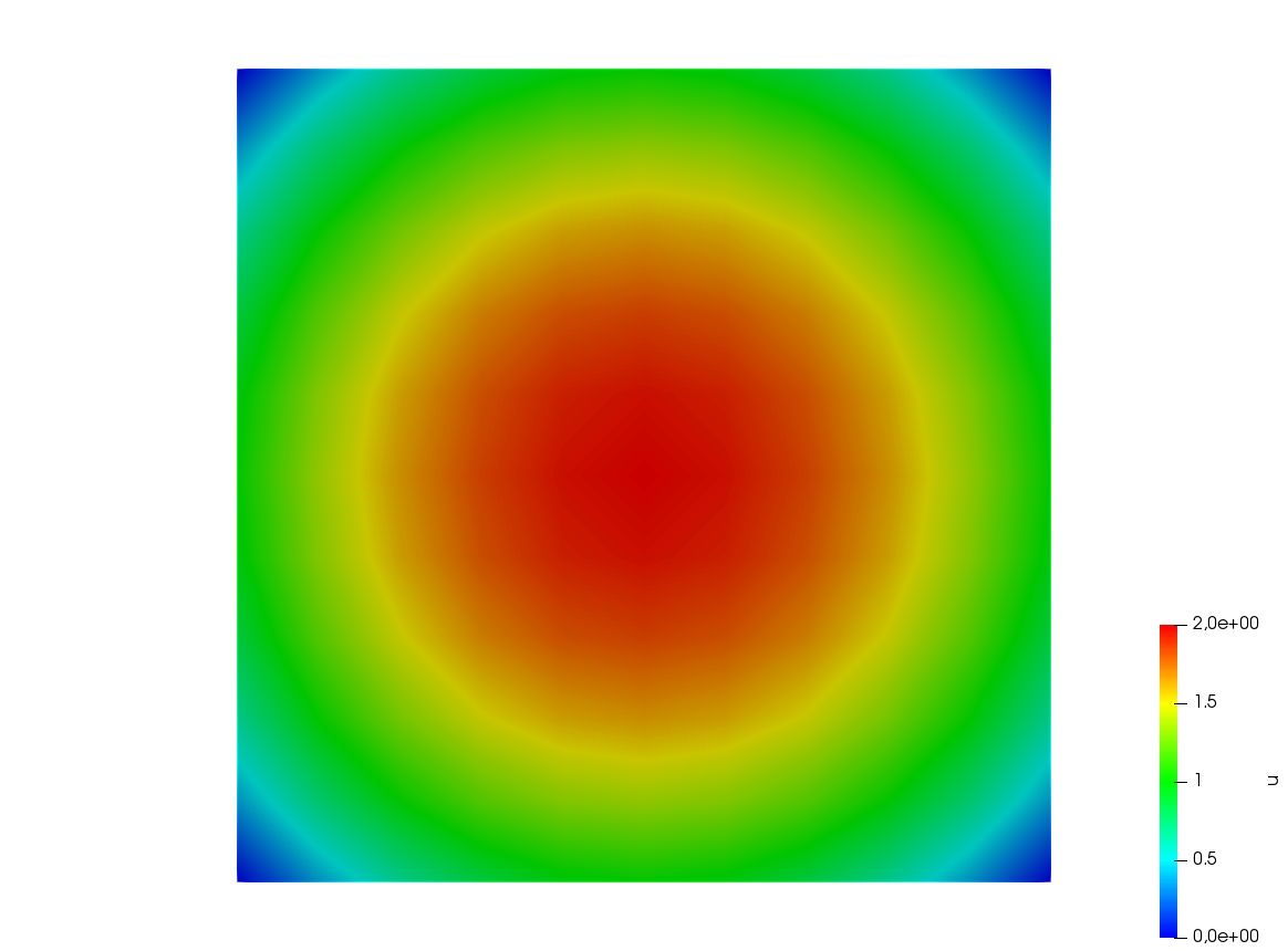
 4// Plot scalar and vectorial FE function
 5Vh uh=x*x+y*y, vh=-y^2+x^2;
 6plot(Th, uh, [uh, vh], value=true, wait=true);
 7
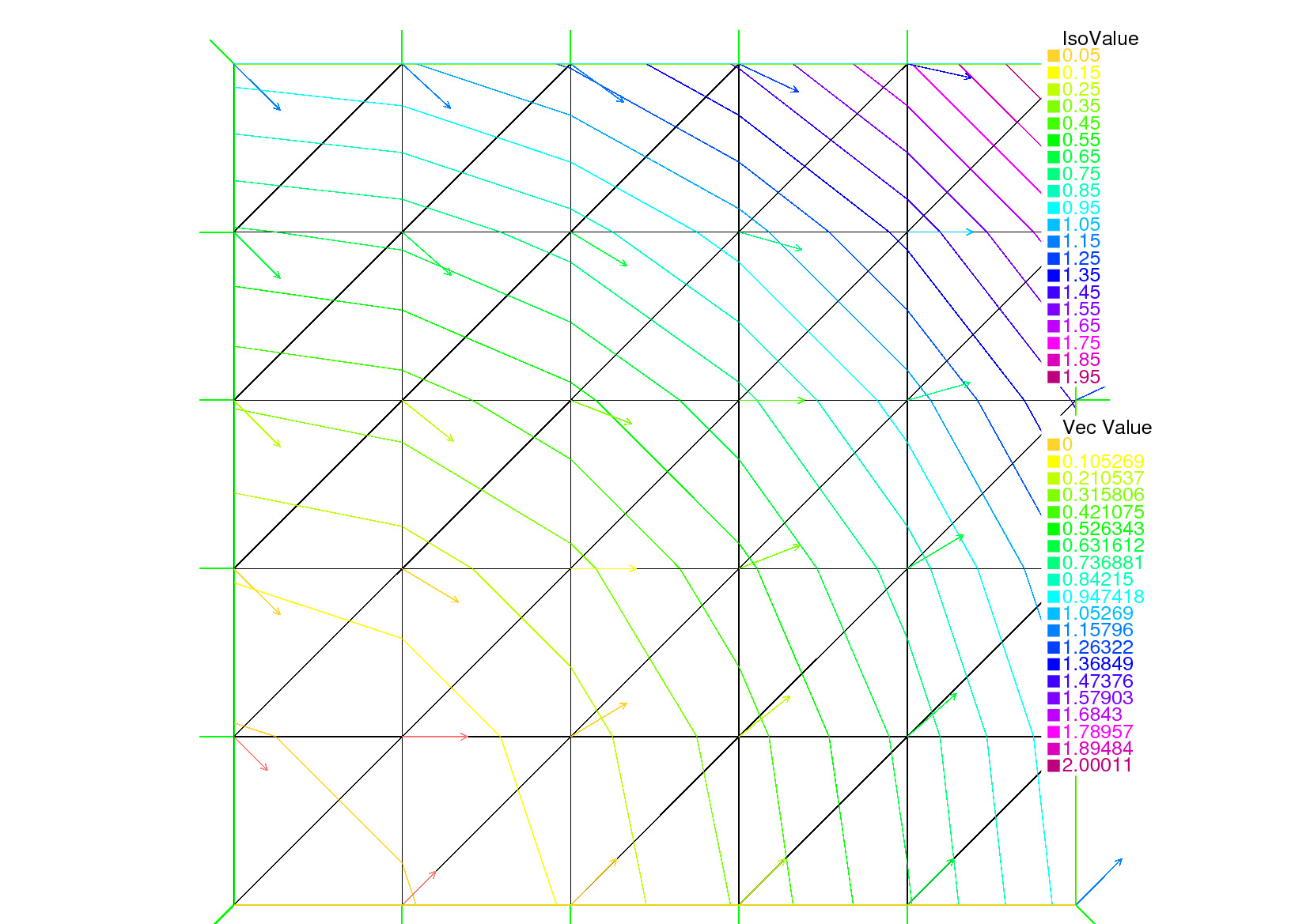
 8// Zoom on box defined by the two corner points [0.1,0.2] and [0.5,0.6]
 9plot(uh, [uh, vh], bb=[[0.1, 0.2], [0.5, 0.6]],
10    wait=true, grey=true, fill=true, value=true);
11
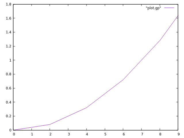
12// Compute a cut
13int n = 10;
14real[int] xx(10), yy(10);
15for (int i = 0; i < n; i++){
16    x = i/real(n);
17    y = i/real(n);
18    xx[i] = i;
19    yy[i] = uh; // Value of uh at point (i/10., i/10.)
20}
21plot([xx, yy], wait=true);
22
23{ // File for gnuplot
24    ofstream gnu("plot.gp");
25    for (int i = 0; i < n; i++)
26        gnu << xx[i] << " " << yy[i] << endl;
27}
28
29// Calls the gnuplot command, waits 5 seconds and generates a postscript plot (UNIX ONLY)
30exec("echo 'plot \"plot.gp\" w l \n pause 5 \n set term postscript \n set output \"gnuplot.eps\" \n replot \n quit' | gnuplot");

 1// From: http://en.wikipedia.org/wiki/HSV_color_space
 2// The HSV (Hue, Saturation, Value) model defines a color space
 3// in terms of three constituent components:
 4// HSV color space as a color wheel
 5// Hue, the color type (such as red, blue, or yellow):
 6// Ranges from 0-360 (but normalized to 0-100% in some applications like here)
 7// Saturation, the "vibrancy" of the color: Ranges from 0-100%
 8// The lower the saturation of a color, the more "grayness" is present
 9// and the more faded the color will appear.
10// Value, the brightness of the color: Ranges from 0-100%
11
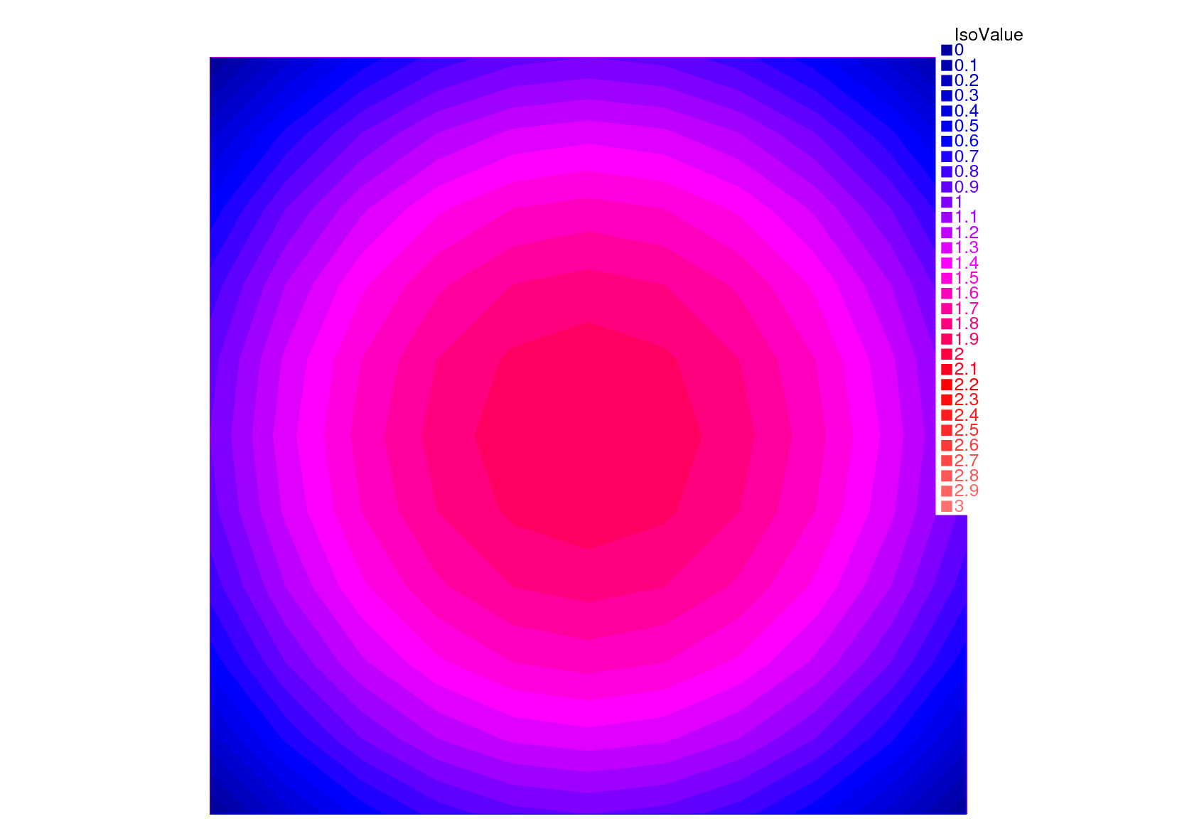
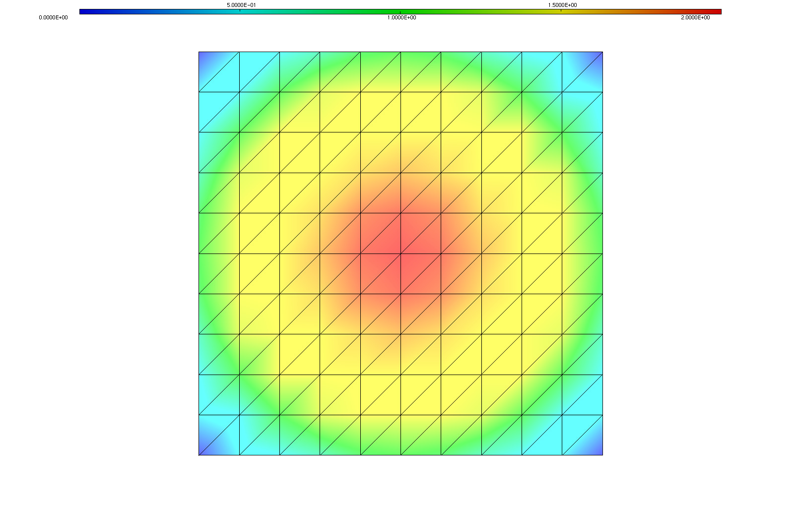
12mesh Th = square(10, 10, [2*x-1, 2*y-1]);
13
14fespace Vh(Th, P1);
15Vh uh=2-x*x-y*y;
16
17real[int] colorhsv=[ // Color hsv model
18    4./6., 1 , 0.5, // Dark blue
19    4./6., 1 , 1, // Blue
20    5./6., 1 , 1, // Magenta
21    1, 1. , 1, // Red
22    1, 0.5 , 1 // Light red
23    ];
24 real[int] viso(31);
25
26 for (int i = 0; i < viso.n; i++)
27    viso[i] = i*0.1;
28
29 plot(uh, viso=viso(0:viso.n-1), value=true, fill=true, wait=true, hsv=colorhsv);

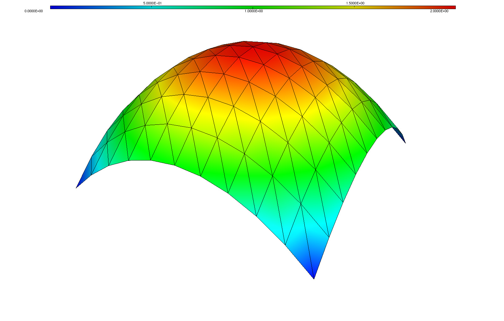
 1load "medit"
 2
 3mesh Th = square(10, 10, [2*x-1, 2*y-1]);
 4
 5fespace Vh(Th, P1);
 6Vh u=2-x*x-y*y;
 7
 8medit("u", Th, u);
 9
10// Old way
11savemesh(Th, "u", [x, y, u*.5]); // Saves u.points and u.faces file
12// build a u.bb file for medit
13{
14    ofstream file("u.bb");
15    file << "2 1 1 " << u[].n << " 2 \n";
16    for (int j = 0; j < u[].n; j++)
17        file << u[][j] << endl;
18}
19// Calls medit command
20exec("ffmedit u");
21// Cleans files on unix-like OS
22exec("rm u.bb u.faces u.points");

 1load "iovtk"
 2
 3mesh Th = square(10, 10, [2*x-1, 2*y-1]);
 4
 5fespace Vh(Th, P1);
 6Vh u=2-x*x-y*y;
 7
 8int[int] Order = [1];
 9string DataName = "u";
10savevtk("u.vtu", Th, u, dataname=DataName, order=Order);