An Example with Complex Numbers
In a microwave oven heat comes from molecular excitation by an electromagnetic field. For a plane monochromatic wave, amplitude is given by Helmholtz’s equation:
\[\beta v + \Delta v = 0.\]
We consider a rectangular oven where the wave is emitted by part of the upper wall. So the boundary of the domain is made up of a part \(\Gamma_1\) where \(v=0\) and of another part \(\Gamma_2=[c,d]\) where for instance \(\displaystyle v=\sin\left(\pi{y-c\over c-d}\right)\).
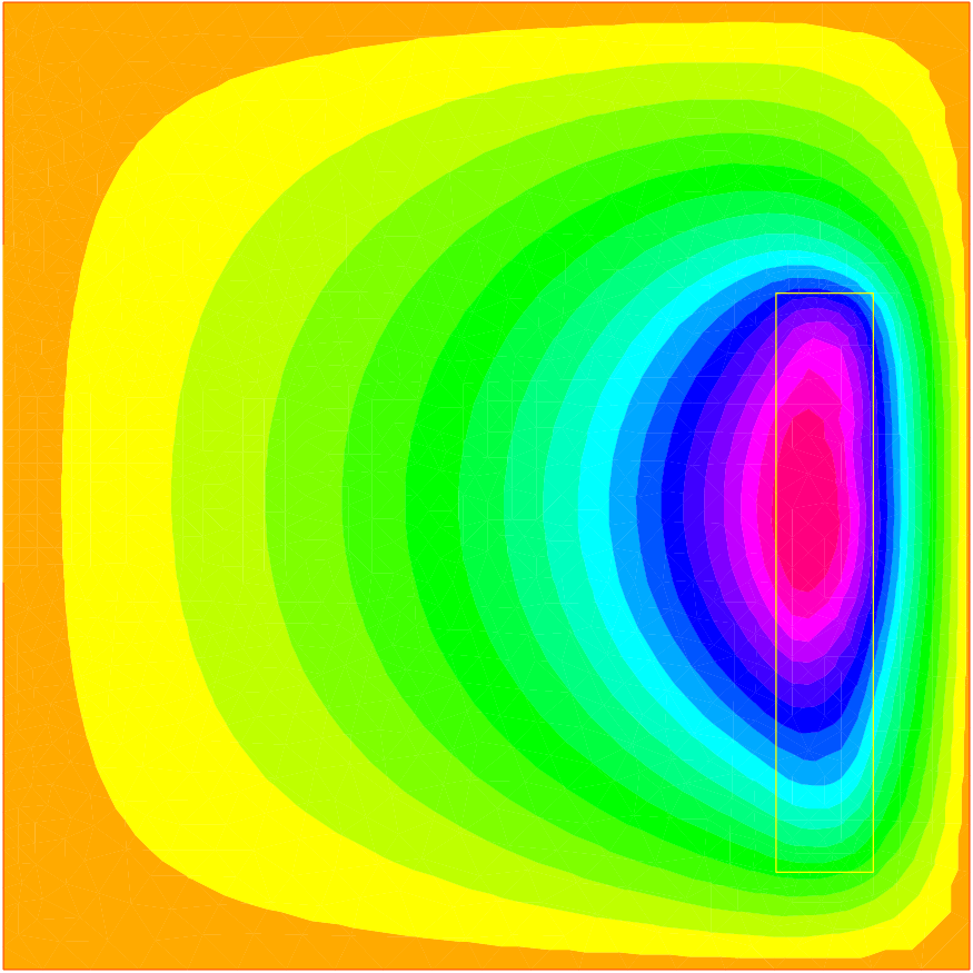
Within an object to be cooked, denoted by \(B\), the heat source is proportional to \(v^2\). At equilibrium, one has :
\[\begin{split}\begin{array}{rcl}
-\Delta\theta &=& v^2 I_B\\
\theta_\Gamma &=& 0
\end{array}\end{split}\]
where \(I_B\) is \(1\) in the object and \(0\) elsewhere.
In the program below \(\beta = 1/(1-i/2)\) in the air and \(2/(1-i/2)\) in the object (\(i=\sqrt{-1}\)):
1// Parameters
2int nn = 2;
3real a = 20.;
4real b = 20.;
5real c = 15.;
6real d = 8.;
7real e = 2.;
8real l = 12.;
9real f = 2.;
10real g = 2.;
11
12// Mesh
13border a0(t=0, 1){x=a*t; y=0; label=1;}
14border a1(t=1, 2){x=a; y=b*(t-1); label=1;}
15border a2(t=2, 3){ x=a*(3-t); y=b; label=1;}
16border a3(t=3, 4){x=0; y=b-(b-c)*(t-3); label=1;}
17border a4(t=4, 5){x=0; y=c-(c-d)*(t-4); label=2;}
18border a5(t=5, 6){x=0; y=d*(6-t); label=1;}
19
20border b0(t=0, 1){x=a-f+e*(t-1); y=g; label=3;}
21border b1(t=1, 4){x=a-f; y=g+l*(t-1)/3; label=3;}
22border b2(t=4, 5){x=a-f-e*(t-4); y=l+g; label=3;}
23border b3(t=5, 8){x=a-e-f; y=l+g-l*(t-5)/3; label=3;}
24
25mesh Th = buildmesh(a0(10*nn) + a1(10*nn) + a2(10*nn) + a3(10*nn) +a4(10*nn) + a5(10*nn)
26 + b0(5*nn) + b1(10*nn) + b2(5*nn) + b3(10*nn));
27real meat = Th(a-f-e/2, g+l/2).region;
28real air= Th(0.01,0.01).region;
29plot(Th, wait=1);
30
31// Fespace
32fespace Vh(Th, P1);
33Vh R=(region-air)/(meat-air);
34Vh<complex> v, w;
35Vh vr, vi;
36
37fespace Uh(Th, P1);
38Uh u, uu, ff;
39
40// Problem
41solve muwave(v, w)
42 = int2d(Th)(
43 v*w*(1+R)
44 - (dx(v)*dx(w) + dy(v)*dy(w))*(1 - 0.5i)
45 )
46 + on(1, v=0)
47 + on(2, v=sin(pi*(y-c)/(c-d)))
48 ;
49
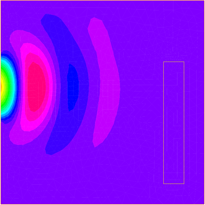
50vr = real(v);
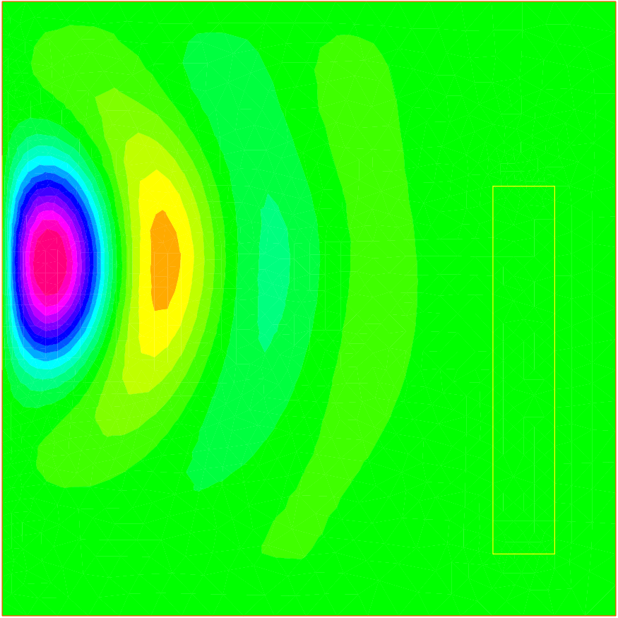
51vi = imag(v);
52
53// Plot
54plot(vr, wait=1, ps="rmuonde.ps", fill=true);
55plot(vi, wait=1, ps="imuonde.ps", fill=true);
56
57// Problem (temperature)
58ff=1e5*(vr^2 + vi^2)*R;
59
60solve temperature(u, uu)
61 = int2d(Th)(
62 dx(u)* dx(uu)+ dy(u)* dy(uu)
63 )
64 - int2d(Th)(
65 ff*uu
66 )
67 + on(1, 2, u=0)
68 ;
69
70// Plot
71plot(u, wait=1, ps="tempmuonde.ps", fill=true);