Evolution problems

FreeFEM also solves evolution problems such as the heat equation:

(60)\[\begin{split}\begin{array}{rcll} \frac{\p u}{\p t}-\mu\Delta u &=& f & \textrm{ in }\Omega\times ]0,T[\\ u(\mathbf{x},0) &=& u_0(\mathbf{x}) & \textrm{ in }\Omega\\ \left(\p u/\p n\right)(\mathbf{x},t) &=& 0 & \textrm{ on }\p\Omega\times ]0,T[ \end{array}\end{split}\]

with a positive viscosity coefficient \(\mu\) and homogeneous Neumann boundary conditions.

We solve (60) by FEM in space and finite differences in time.

We use the definition of the partial derivative of the solution in the time derivative:

\[\frac{\p u}{\p t}(x,y,t) = \lim_{\tau \to 0}\frac{u(x,y,t)-u(x,y,t-\tau )}{\tau }\]

which indicates that \(u^m(x,y)=u(x,y,m\tau )\) will satisfy approximatively:

\[\frac{\p u}{\p t}(x,y,m\tau )\simeq \frac{u^m(x,y)-u^{m-1}(x,y)}{\tau }\]

The time discretization of heat equation (60) is as follows, \(\forall m=0,\cdots,[T/\tau ]\):

\[\begin{split}\begin{array}{rcll} \frac{u^{m+1}-u^{m}}{\tau }-\mu\Delta u^{m+1} &=& f^{m+1} & \textrm{ in }\Omega\\ u^0(\mathbf{x}) &=& u_0(\mathbf{x}) & \textrm{ in }\Omega\\ \p u^{m+1}/\p n(\mathbf{x}) &=& 0 & \textrm{ on }\p\Omega \end{array}\end{split}\]

which is so-called backward Euler method for (60).

To obtain the variational formulation, multiply with the test function \(v\) both sides of the equation:

\[\int_{\Omega}\{u^{m+1}v-\tau \Delta u^{m+1}v\}=\int_{\Omega}\{u^m+\tau f^{m+1}\}v\]

By the divergence theorem, we have:

\[\int_{\Omega}\{u^{m+1}v+\tau\nabla u^{m+1}\cdot \nabla v\} -\int_{\p\Omega} \tau \left( \p u^{m+1}/\p n\right) v =\int_{\Omega }\{u^mv+\tau f^{m+1}v\}\]

By the boundary condition \(\p u^{m+1}/\p n=0\), it follows that:

(61)\[\int_{\Omega} \{u^{m+1}v+\tau \nabla u^{m+1}\cdot \nabla v\} -\int_{\Omega }\{u^mv+\tau f^{m+1}v\} =0\]

Using the identity just above, we can calculate the finite element approximation \(u_h^m\) of \(u^m\) in a step-by-step manner with respect to \(t\).

Tip

Example

We now solve the following example with the exact solution \(u(x,y,t)=tx^4\), \(\Omega = ]0,1[^2\).

\[\begin{split}\begin{array}{rcll} \frac{{\p u}}{{\p t}} - \mu \Delta u &=& x^4 - \mu 12tx^2 & \textrm{ in }\Omega\times ]0,3[\\ u(x,y,0) &=& 0 & \textrm{ on }\Omega\\ \left. u \right|_{\p\Omega} &=& t*x^4 \end{array}\end{split}\]

// Parameters
real dt = 0.1;
real mu = 0.01;

// Mesh
mesh Th = square(16, 16);

// Fespace
fespace Vh(Th, P1);
Vh u, v, uu, f, g;

// Problem
problem dHeat (u, v)
    = int2d(Th)(
          u*v
        + dt*mu*(dx(u)*dx(v) + dy(u)*dy(v))
    )
    + int2d(Th)(
        - uu*v
        - dt*f*v
    )
    + on(1, 2, 3, 4, u=g)
    ;

// Time loop
real t = 0;
uu = 0;
for (int m = 0; m <= 3/dt; m++){
    // Update
    t = t+dt;
    f = x^4 - mu*t*12*x^2;
    g = t*x^4;
    uu = u;

    // Solve
    dHeat;

    // Plot
    plot(u, wait=true);
    cout << "t=" << t << " - L^2-Error=" << sqrt(int2d(Th)((u-t*x^4)^2)) << endl;
}

In the last statement, the \(L^2\)-error \(\left(\int_{\Omega}\left| u-tx^4\right|^2\right)^{1/2}\) is calculated at \(t=m\tau, \tau =0.1\). At \(t=0.1\), the error is 0.000213269. The errors increase with \(m\) and 0.00628589 at \(t=3\).

The iteration of the backward Euler (61) is made by for loop.

Note

The stiffness matrix in the loop is used over and over again. FreeFEM support reuses of stiffness matrix.

Mathematical Theory on Time Difference Approximations.

In this section, we show the advantage of implicit schemes. Let \(V, H\) be separable Hilbert space and \(V\) is dense in \(H\). Let \(a\) be a continuous bilinear form over \(V \times V\) with coercivity and symmetry.

Then \(\sqrt{a(v,v)}\) become equivalent to the norm \(\| v\|\) of \(V\).

Problem Ev(f,Omega): For a given \(f\in L^2(0,T;V'),\, u^0\in H\)

\[\begin{split}\begin{array}{rcl} \frac{d}{dt}(u(t),v)+a(u(t),v)&=&( f(t),v)\qquad \forall v\in V,\quad a.e. \, t\in [0,T]\\ u(0)&=&u^0\nonumber \end{array}\end{split}\]

where \(V'\) is the dual space of \(V\).

Then, there is an unique solution \(u\in L^{\infty}(0,T;H)\cap L^2(0,T;V)\).

Let us denote the time step by \(\tau>0\), \(N_T=[T/\tau]\). For the discretization, we put \(u^n = u(n\tau)\) and consider the time difference for each \(\theta\in [0,1]\)

(62)\[\begin{split}\begin{array}{rcl} \frac{1}{\tau}\left( u_h^{n+1}-u_h^n,\phi_i\right) +a\left( u_h^{n+\theta},\phi_i\right)&=&\langle f^{n+\theta},\phi_i\rangle\\ i=1,&\cdots&, m,\quad n=0,\cdots, N_T\nonumber\\ u_h^{n+\theta}&=&\theta u_h^{n+1}+(1-\theta)u_h^n,\\ f^{n+\theta}&=&\theta f^{n+1}+(1-\theta)f^n\nonumber \end{array}\end{split}\]

Formula (62) is the forward Euler scheme if \(\theta=0\), Crank-Nicolson scheme if \(\theta=1/2\), the backward Euler scheme if \(\theta=1\).

Unknown vectors \(u^n=(u_h^1,\cdots,u_h^M)^T\) in

\[u_h^n(x)=u^n_1\phi_1(x)+\cdots+u^n_m\phi_m(x),\quad u^n_1,\cdots,u^n_m\in \R\]

are obtained from solving the matrix

(63)\[\begin{split}(M+\theta\tau A)u^{n+1}=\{M-(1-\theta)\tau A\}u^n +\tau\left\{\theta f^{n+1}+(1-\theta)f^n\right\}\\ M=(m_{ij}),\quad m_{ij}=(\phi_j,\phi_i),\qquad A=(a_{ij}),\quad a_{ij}=a(\phi_j,\phi_i)\nonumber\end{split}\]

Refer [TABATA1994], pp.70–75 for solvability of (63). The stability of (63) is in [TABATA1994], Theorem 2.13:

Let \(\{\mathcal{T}_h\}_{h\downarrow 0}\) be regular triangulations (see Regular Triangulation). Then there is a number \(c_0>0\) independent of \(h\) such that,

\[\begin{split}|u_h^n|^2\le \left\{ \begin{array}{lr} \frac{1}{\delta}\left\{ |u^0_h|^2+\tau \sum_{k=0}^{n-1}\|f^{k+\theta}\|^2_{V_h'} \right\}&\theta\in [0,1/2)\\ |u^0_h|^2+\tau \sum_{k=0}^{n-1}\|f^{k+\theta}\|^2_{V_h'}&\theta\in [1/2,1] \end{array} \right.\end{split}\]

if the following are satisfied:

When \(\theta\in [0,1/2)\), then we can take a time step \(\tau\) in such a way that

\[\tau <\frac{2(1-\delta)}{(1-2\theta)c_0^2}h^2\]

for arbitrary \(\delta\in (0,1)\).
When \(1/2\leq \theta\leq 1\), we can take \(\tau\) arbitrary.

Tip

Example

// Parameters
real tau = 0.1; real
theta = 0.;

// Mesh
mesh Th = square(12, 12);

// Fespace
fespace Vh(Th, P1);
Vh u, v, oldU;
Vh f1, f0;

fespace Ph(Th, P0);
Ph h = hTriangle; // mesh sizes for each triangle

// Function
func real f (real t){
    return x^2*(x-1)^2 + t*(-2 + 12*x - 11*x^2 - 2*x^3 + x^4);
}

// File
ofstream out("err02.csv"); //file to store calculations
out << "mesh size = " << h[].max << ", time step = " << tau << endl;
for (int n = 0; n < 5/tau; n++)
    out << n*tau << ",";
out << endl;

// Problem
problem aTau (u, v)
    = int2d(Th)(
          u*v
        + theta*tau*(dx(u)*dx(v) + dy(u)*dy(v) + u*v)
    )
    - int2d(Th)(
          oldU*v
        - (1-theta)*tau*(dx(oldU)*dx(v) + dy(oldU)*dy(v) + oldU*v)
    )
    - int2d(Th)(
          tau*(theta*f1 + (1-theta)*f0)*v
    )
    ;

// Theta loop
while (theta <= 1.0){
    real t = 0;
    real T = 3;
    oldU = 0;
    out << theta << ",";
    for (int n = 0; n < T/tau; n++){
        // Update
        t = t + tau;
        f0 = f(n*tau);
        f1 = f((n+1)*tau);

        // Solve
        aTau;
        oldU = u;

        // Plot
        plot(u);

        // Error
        Vh uex = t*x^2*(1-x)^2; //exact solution = tx^2(1-x)^2
        Vh err = u - uex; // err = FE-sol - exact
        out << abs(err[].max)/abs(uex[].max) << ",";
    }
    out << endl;
    theta = theta + 0.1;
}

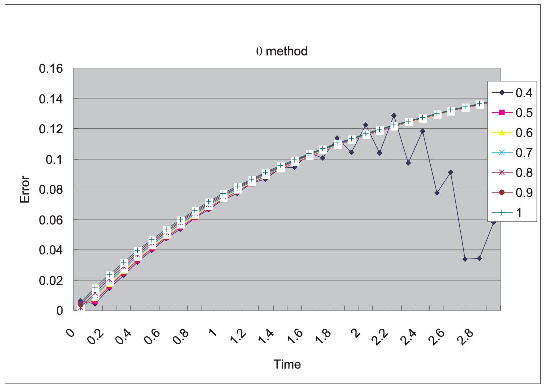
../_images/EvolutionProblems_TimeDifference.png — Fig. 161 \(\max_{x\in\Omega}\vert u_h^n(\theta)-u_{ex}(n\tau)\vert\max_{x\in\Omega}\vert u_{ex}(n\tau)\vert at n=0,1,\cdots,29\)

We can see in Fig. 161 that \(u_h^n(\theta)\) become unstable at \(\theta=0.4\), and figures are omitted in the case \(\theta<0.4\).

Convection

The hyperbolic equation

(64)\[\p_t u +\mathbf{\alpha} \cdot \nabla u=f;\ \textrm{ for a vector-valued function }\mathbf{\alpha}\]

appears frequently in scientific problems, for example in the Navier-Stokes equations, in the Convection-Diffusion equation, etc.

In the case of 1-dimensional space, we can easily find the general solution \((x,t)\mapsto u(x,t)=u^0(x-\alpha t)\) of the following equation, if \(\alpha\) is constant,

(65)\[\begin{split}\begin{array}{rcl} \p_t u +\alpha\p_x u &=& 0\\ u(x,0) &=& u^0(x), \end{array}\end{split}\]

because \(\p_t u +\alpha\p_x u=-\alpha\dot{u}^0+a\dot{u}^0=0\), where \(\dot{u}^0=du^0(x)/dx\).

Even if \(\alpha\) is not constant, the construction works on similar principles. One begins with the ordinary differential equation (with the convention that \(\alpha\) is prolonged by zero apart from \((0,L)\times (0,T)\)):

\[\dot{X}(\tau )=+\alpha(X(\tau ),\tau ),\ \tau \in (0,t)\quad X(t)=x\]

In this equation \(\tau\) is the variable and \(x,t\) are parameters, and we denote the solution by \(X_{x,t}(\tau )\). Then it is noticed that \((x,t)\rightarrow v(X(\tau),\tau)\) in \(\tau=t\) satisfies the equation

\[\p _{t}v+\alpha\p _{x}v=\p _{t}X\dot{v}+a\p _{x}X\dot{v}% =0\]

and by the definition \(\p _{t}X=\dot{X}=+\alpha\) and \(\p_{x}X=\p _{x}x\) in \(\tau=t\), because if \(\tau =t\) we have \(X(\tau )=x\).

The general solution of (65) is thus the value of the boundary condition in \(X_{x, t}(0)\), that is to say \(u(x,t)=u^{0}(X_{x,t}(0))\) where \(X_{x,t}(0)\) is on the \(x\) axis, \(u(x,t)=u^{0}(X_{x,t}(0))\) if \(X_{x,t}(0)\) is on the axis of \(t\).

In higher dimension \(\Omega \subset R^{d},~d=2,3\), the equation for the convection is written

\[\p _{t}u+\mathbf{\alpha}\cdot \nabla u=0\hbox{ in }\Omega \times (0,T)\]

where \(\mathbf{a}(x,t)\in \R^{d}\).

FreeFEM implements the Characteristic-Galerkin method for convection operators. Recall that the equation (64) can be discretized as

\[\frac{Du}{Dt} = f\;\;\textrm{i.e. }\frac{du}{dt}\left( {X(t),t} \right) = f\left(X( t ),t \right)\textrm{ where }\frac{dX}{dt}( t ) = \mathbf{\alpha}( {X(t),t})\]

where \(D\) is the total derivative operator. So a good scheme is one step of backward convection by the method of Characteristics-Galerkin

(66)\[\frac{1}{{\tau }}\left(u^{m + 1}(x) - u^m(X^m(x))\right) = f^{m+1} (x)\]

where \(X^m (x)\) is an approximation of the solution at \(t = m\tau\) of the ordinary differential equation

\[\frac{d\mathbf{X}}{dt}(t) = \mathbf{\alpha}^m(\mathbf{X}(t)), \mathbf{X}((m + 1)\tau) = x.\]

where \(\mathbf{\alpha}^m(x)=(\alpha_1(x,m\tau ),\alpha_2(x,m\tau))\). Because, by Taylor’s expansion, we have

(67)\[\begin{split}\begin{array}{rcl} u^m(\mathbf{X}(m\tau ))&=& u^m(\mathbf{X}((m+1)\tau )) - \tau \sum_{i=1}^d \frac{\p u^m}{\p x_i}(\mathbf{X}((m+1)\tau )) \frac{\p X_i}{\p t}((m+1)\tau ) +o(\tau )\nonumber\\ &=&u^m(x)-\tau \mathbf{\alpha}^m(x)\cdot \nabla u^m(x)+o(\tau ) \end{array}\end{split}\]

where \(X_i(t)\) are the i-th component of \(\mathbf{X}(t)\), \(u^m(x)=u(x,m\tau )\) and we used the chain rule and \(x=\mathbf{X}((m+1)\tau )\). From (67), it follows that

\[u^m(X^m(x))=u^m(x)-\tau \mathbf{\alpha}^m(x)\cdot \nabla u^m(x)+o(\tau )\]

Also we apply Taylor’s expansion for \(t \rightarrow u^m(x-\mathbf{\alpha}^m(x)t),0\le t\le \tau\), then

\[u^m(x-\mathbf{\alpha}\tau )=u^m(x)-\tau \mathbf{\alpha}^m(x)\cdot \nabla u^m(x)+o(\tau ).\]

Putting

convect\(\left( {\mathbf{\alpha},-\tau ,u^m } \right)\approx u^m \left(x - \mathbf{\alpha}^m\tau \right)\)

we can get the approximation

\(u^m \left( {X^m( x )} \right) \approx\) convect \(\left( {[a_1^m ,a_2^m],-\tau ,u^m } \right)\) by \(X^m \approx x \mapsto x- \tau [a_1^m(x) ,a_2^m(x)]\)

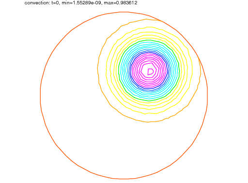
A classical convection problem is that of the “rotating bell” (quoted from [LUCQUIN1998], p.16).

Let \(\Omega\) be the unit disk centered at 0, with its center rotating with speed \(\alpha_1 = y,\, \alpha_2 = -x\). We consider the problem (64) with \(f=0\) and the initial condition \(u(x,0)=u^0(x)\), that is, from (66)

\(u^{m + 1}(x) = u^m(X^m(x))\approx\) convect\((\mathbf{\alpha},-\tau ,u^m)\)

The exact solution is \(u(x, t) = u(\mathbf{X}(t))\) where \(\mathbf{X}\) equals \(x\) rotated around the origin by an angle \(\theta = -t\) (rotate in clockwise). So, if \(u^0\) in a 3D perspective looks like a bell, then \(u\) will have exactly the same shape, but rotated by the same amount. The program consists in solving the equation until \(T = 2\pi\), that is for a full revolution and to compare the final solution with the initial one; they should be equal.

Tip

Convect

// Parameters
real dt = 0.17;

// Mesh
border C(t=0, 2*pi){x=cos(t); y=sin(t);}
mesh Th = buildmesh(C(70));

// Fespace
fespace Vh(Th, P1);
Vh u0;
Vh a1 = -y, a2 = x; //rotation velocity
Vh u;

// Initialization
u = exp(-10*((x-0.3)^2 +(y-0.3)^2));

// Time loop
real t = 0.;
for (int m = 0; m < 2*pi/dt; m++){
    // Update
    t += dt;
    u0 = u;

    // Convect
    u = convect([a1, a2], -dt, u0); //u^{m+1}=u^m(X^m(x))

    // Plot
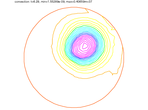
    plot(u, cmm=" t="+t+", min="+u[].min+", max="+u[].max);
}

Note

The scheme convect is unconditionally stable, then the bell become lower and lower (the maximum of \(u^{37}\) is \(0.406\) as shown in Fig. 162.

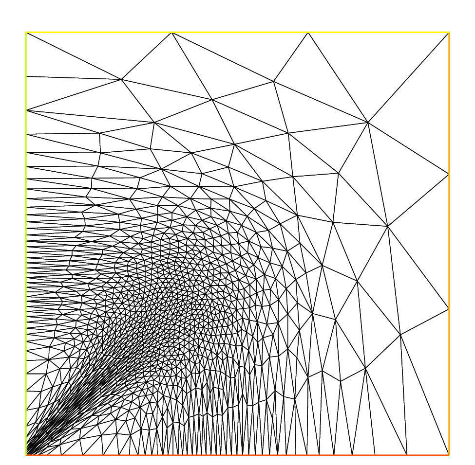
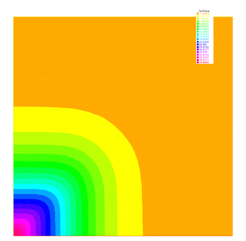
EvolutionProblem_Convect — Fig. 162 \(u^0=e^{-10((x-0.3)^2 +(y-0.3)^2)}\)

EvolutionProblem_Convect2 — Fig. 163 The bell at \(t=6.29\)

2D Black-Scholes equation for an European Put option

In mathematical finance, an option on two assets is modeled by a Black-Scholes equations in two space variables, (see for example [WILMOTT1995] or [ACHDOU2005]).

\[\begin{split}\begin{array}{rcl} \p _t u &+& \frac{{\left( {\sigma _1 x } \right)^2 }}{2}\frac{{\p ^2 u}}{{\p x^2 }} + \frac{{\left( {\sigma _2 y } \right)^2 }}{2}\frac{{\p ^2 u}}{{\p y^2 }} \\ &&{\rm{ }} + \rho x y \frac{{\p ^2 u}}{{\p x \p y }} + rS_1 \frac{{\p u}}{{\p x }} + rS_2 \frac{{\p u}}{{\p y }} - rP = 0 \nonumber \end{array}\end{split}\]

which is to be integrated in \(\left( {0,T} \right) \times \R^ + \times \R^ +\) subject to, in the case of a put

\[u\left( {x , y ,T} \right) = \left( {K - \max \left( {x ,y } \right)} \right)^+\]

Boundary conditions for this problem may not be so easy to device. As in the one dimensional case the PDE contains boundary conditions on the axis \(x_1 = 0\) and on the axis \(x_2 = 0\), namely two one dimensional Black-Scholes equations driven respectively by the data \(u\left( {0, + \infty ,T} \right)\) and \(u\left( { + \infty ,0,T} \right)\). These will be automatically accounted for because they are embedded in the PDE. So if we do nothing in the variational form (i.e. if we take a Neumann boundary condition at these two axis in the strong form) there will be no disturbance to these. At infinity in one of the variable, as in 1D, it makes sense to impose \(u=0\). We take

\[\sigma _1 = 0.3,\;\;\sigma _2 = 0.3,\;\;\rho = 0.3,\;\;r = 0.05,\;\;K = 40,\;\;T = 0.5\]

An implicit Euler scheme is used and a mesh adaptation is done every 10 time steps. To have an unconditionally stable scheme, the first order terms are treated by the Characteristic Galerkin method, which, roughly, approximates

\[\frac{{\p u}}{{\p t}} + a_1 \frac{{\p u}}{{\p x}} + a_2 \frac{{\p u}}{{\p y}} \approx \frac{1}{{\tau }}\left( {u^{n + 1} \left( x \right) - u^n \left( {x - \mathbf{\alpha}\tau } \right)} \right)\]

Tip

Black-Scholes

// Parameters
int m = 30; int L = 80; int LL = 80; int j = 100; real sigx = 0.3; real sigy = 0.3; real rho = 0.3; real r = 0.05; real K = 40; real dt = 0.01;

// Mesh
mesh th = square(m, m, [L*x, LL*y]);

// Fespace
fespace Vh(th, P1);
Vh u = max(K-max(x,y),0.);
Vh xveloc, yveloc, v, uold;

// Time loop
for (int n = 0; n*dt <= 1.0; n++){
    // Mesh adaptation
    if (j > 20){
        th = adaptmesh(th, u, verbosity=1, abserror=1, nbjacoby=2,
        err=0.001, nbvx=5000, omega=1.8, ratio=1.8, nbsmooth=3,
        splitpbedge=1, maxsubdiv=5, rescaling=1);
        j = 0;
        xveloc = -x*r + x*sigx^2 + x*rho*sigx*sigy/2;
        yveloc = -y*r + y*sigy^2 + y*rho*sigx*sigy/2;
        u = u;
    }

    // Update
    uold = u;

    // Solve
    solve eq1(u, v, init=j, solver=LU)
        = int2d(th)(
              u*v*(r+1/dt)
            + dx(u)*dx(v)*(x*sigx)^2/2
            + dy(u)*dy(v)*(y*sigy)^2/2
            + (dy(u)*dx(v) + dx(u)*dy(v))*rho*sigx*sigy*x*y/2
        )
        - int2d(th)(
              v*convect([xveloc, yveloc], dt, uold)/dt
        )
        + on(2, 3, u=0)
        ;

    // Update
    j = j+1;
};

// Plot
plot(u, wait=true, value=true);

Results are shown on Fig. 164 and Fig. 165.

EvolutionProblems_BlackSholes — Fig. 164 The adapted triangulation

EvolutionProblems_BlackSholes2 — Fig. 165 The level line of the European basquet put option

Here you can use the search bar to search in all FreeFEM examples instead

The list of all matching examples on the right is updated for each new query

Clicking on a search hit or on an example on the right brings up the corresponding script from GitHub

You can also filter the list on the right by selecting one or more intersecting categories on the left tree