A Large Fluid Problem

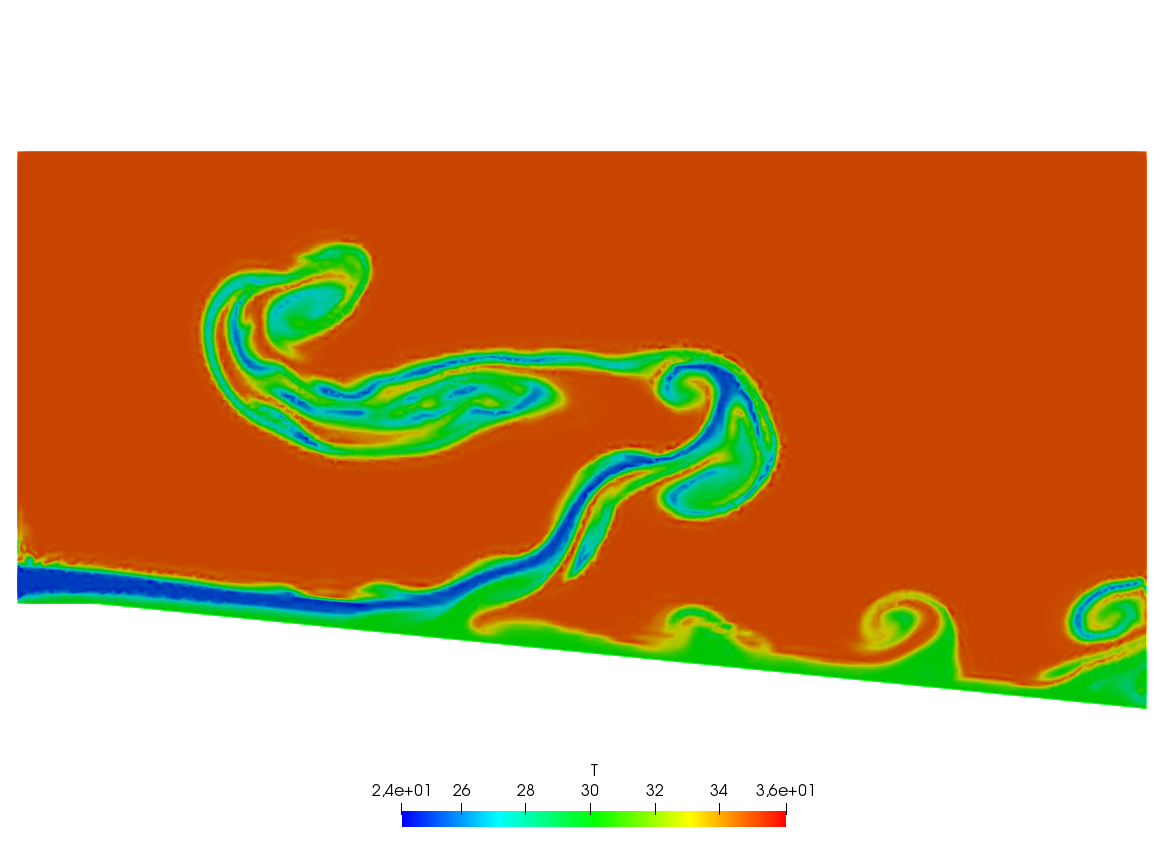
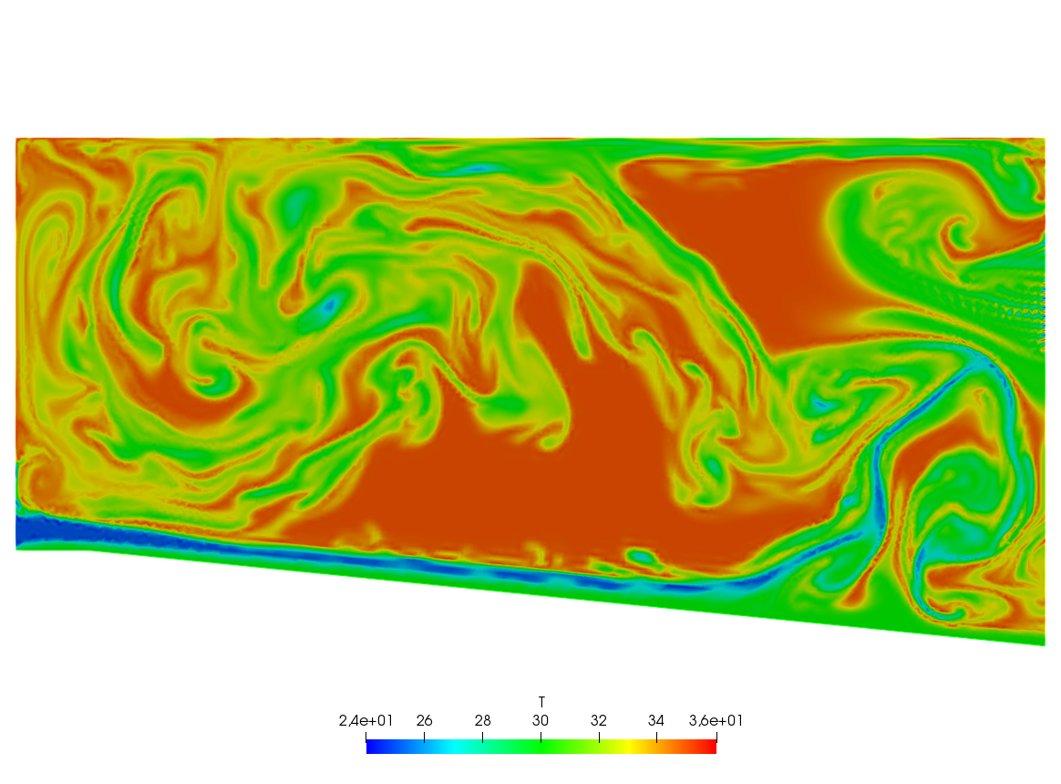
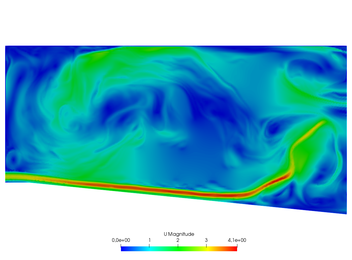
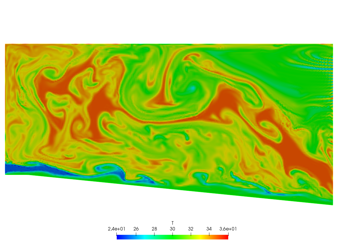
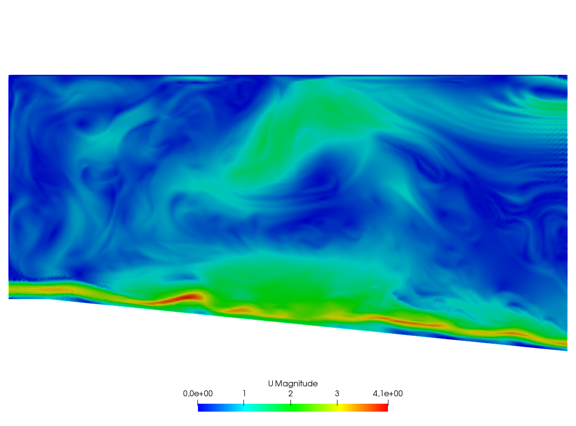
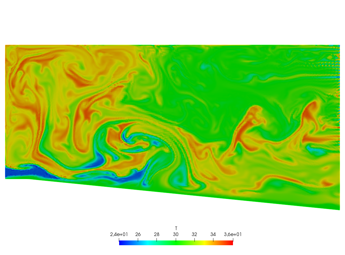
A friend of one of us in Auroville-India was building a ramp to access an air conditioned room. As I was visiting the construction site he told me that he expected to cool air escaping by the door to the room to slide down the ramp and refrigerate the feet of the coming visitors. I told him “no way” and decided to check numerically.

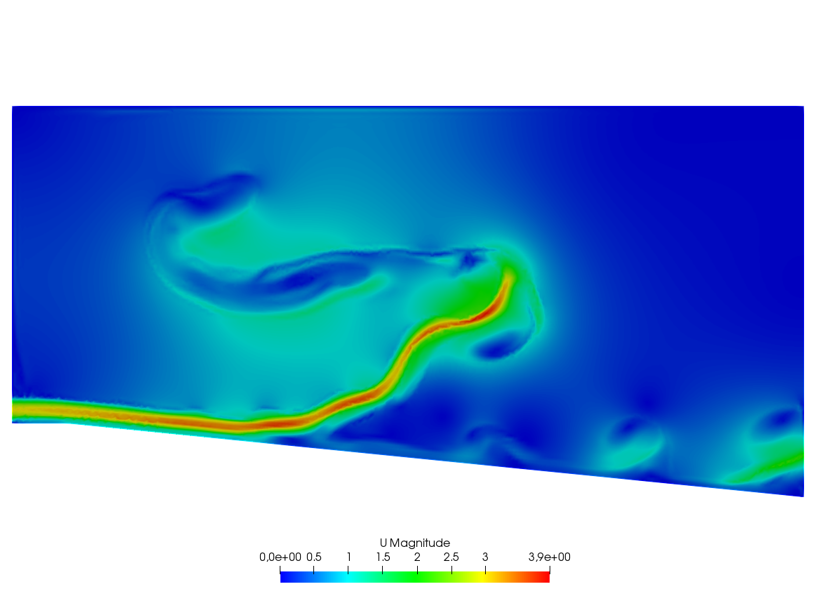
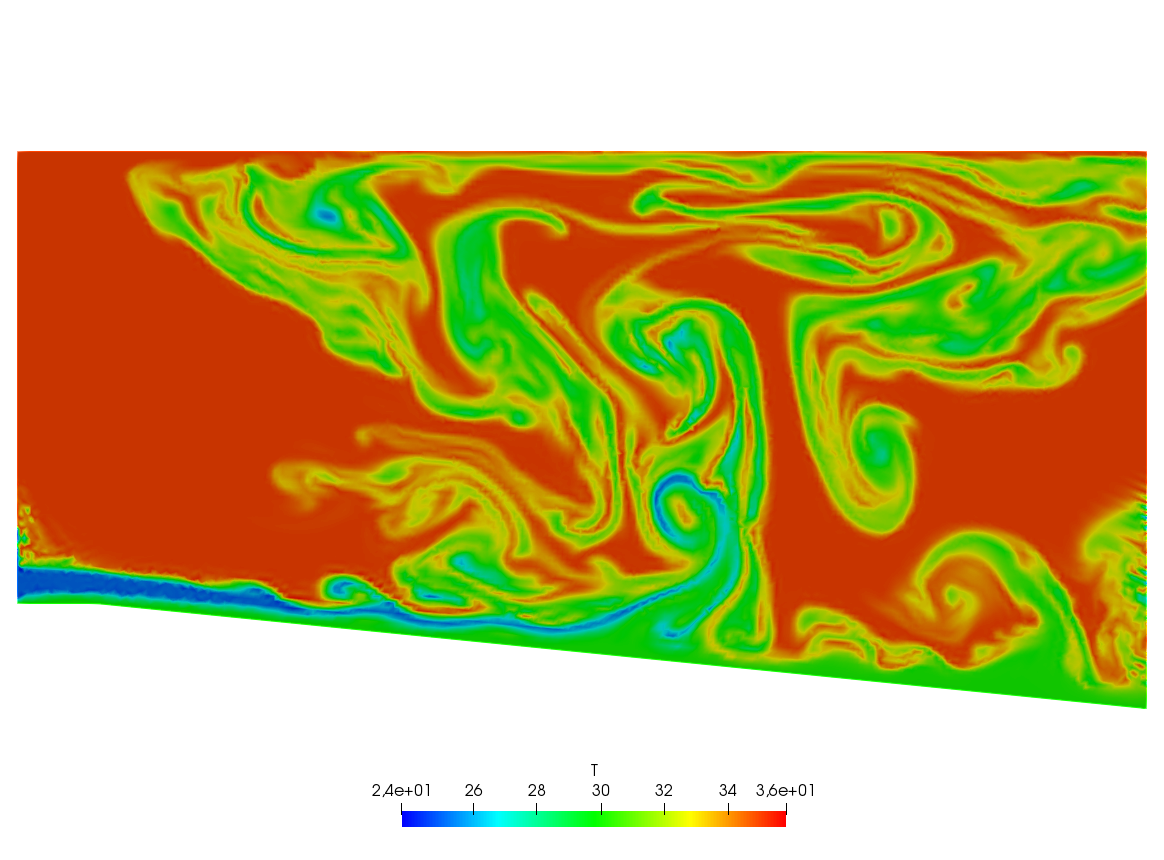
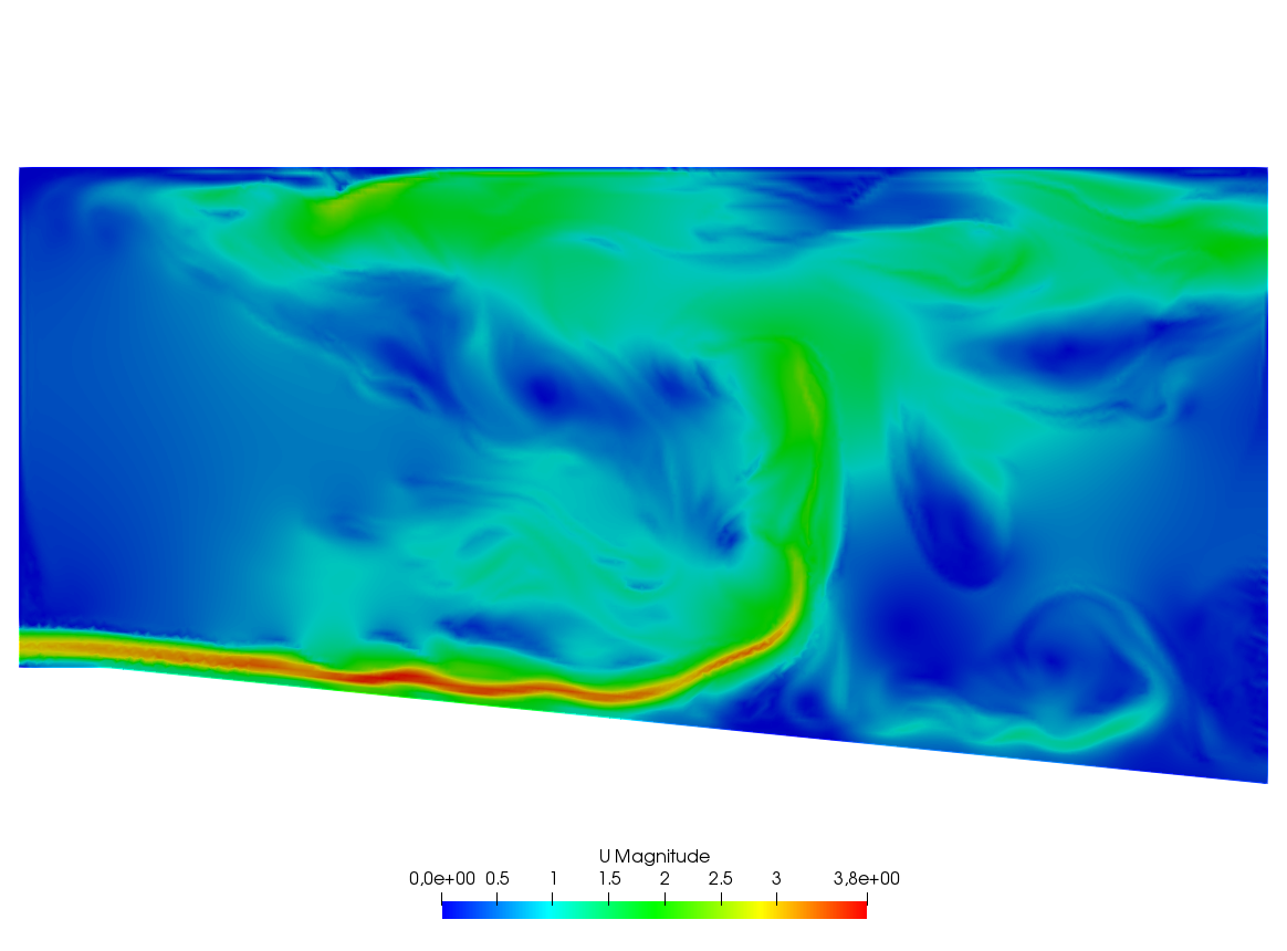
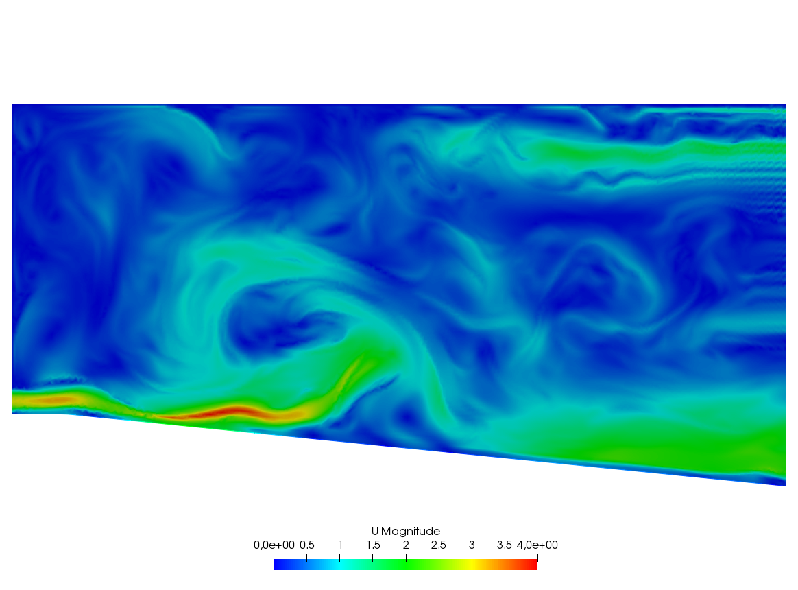
The fluid velocity and pressure are solution of the Navier-Stokes equations with varying density function of the temperature.

The geometry is trapezoidal with prescribed inflow made of cool air at the bottom and warm air above and so are the initial conditions; there is free outflow, slip velocity at the top (artificial) boundary and no-slip at the bottom. However the Navier-Stokes cum temperature equations have a RANS \(k-\epsilon\) model and a Boussinesq approximation for the buoyancy. This comes to :

\[\begin{split}\begin{array}{rcl} \partial_t\theta+u\nabla\theta-\nabla\cdot(\kappa_T^m\nabla\theta) &=& 0\\ \partial_t u +u\nabla u -\nabla\cdot(\mu_T\nabla u) +\nabla p+ e(\theta-\theta_0)\vec e_2 &=&0\\ \nabla\cdot u &=& 0\\ \mu_T &=& c_\mu\frac{k^2}\epsilon\\ \kappa_T &=& \kappa\mu_T\\ \partial_t k + u\nabla k + \epsilon -\nabla\cdot(\mu_T\nabla k) &=& \frac{\mu_T}2|\nabla u+\nabla u^T|^2\\ \partial_t\epsilon+u\nabla\epsilon + c_2\frac{\epsilon^2} k -\frac{c_\epsilon}{c_\mu}\nabla\cdot (\mu_T\nabla\epsilon) &=& \frac{c_1}2 k|\nabla u+\nabla u^T|^2\\ \end{array}\end{split}\]

We use a time discretization which preserves positivity and uses the method of characteristics (\(X^m(x)\approx x-u^m(x)\delta t\))

\[\begin{split}\begin{array}{rcl} \frac 1{\delta t}(\theta^{m+1}-\theta^m \circ X^m)-\nabla\cdot(\kappa_T^m\nabla\theta^{m+1}) &=& 0\\ \frac1{\delta t}(u^{m+1}-u^m \circ X^m) -\nabla\cdot(\mu_T^m\nabla u^{m+1}) +\nabla p^{m+1}+ e(\theta^{m+1}-\theta_0)\vec e_2 &=& 0\\ \nabla\cdot u^{m+1} &=& 0\\ \frac1{\delta t}(k^{m+1}-k^m \circ X^m) + k^{m+1}\frac{\epsilon^m}{k^m} -\nabla\cdot(\mu_T^m\nabla k^{m+1}) &=& \frac{\mu_T^m}2|\nabla u^m+{\nabla u^m}^T|^2\\ \frac1{\delta t}(\epsilon^{m+1}-\epsilon^m \circ X^m) + c_2\epsilon^{m+1}\frac{\epsilon^m} {k^m} -\frac{c_\epsilon}{c_\mu}\nabla\dot(\mu_T^m\nabla\epsilon^{m+1}) &=& \frac{c_1}2 k^m|\nabla u^m+{\nabla u^m}^T|^2\\ \mu_T ^{m+1} &=& c_\mu\frac{{k^{m+1}}^2}{\epsilon^{m+1}}\\ \kappa_T^{m+1} &=& \kappa\mu_T^{m+1} \end{array}\end{split}\]

In variational form and with appropriated boundary conditions the problem is :

load "iovtk"

verbosity=0;

// Parameters
int nn = 15;
int nnPlus = 5;
real l = 1.;
real L = 15.;
real hSlope = 0.1;
real H = 6.;
real h = 0.5;

real reylnods =500;
real beta = 0.01;

real eps = 9.81/303.;
real nu = 1;
real numu = nu/sqrt(0.09);
real nuep = pow(nu,1.5)/4.1;
real dt = 0.;

real Penalty = 1.e-6;

// Mesh
border b1(t=0, l){x=t; y=0;}
border b2(t=0, L-l){x=1.+t; y=-hSlope*t;}
border b3(t=-hSlope*(L-l), H){x=L; y=t;}
border b4(t=L, 0){x=t; y=H;}
border b5(t=H, h){x=0; y=t;}
border b6(t=h, 0){x=0; y=t;}

mesh Th=buildmesh(b1(nnPlus*nn*l) + b2(nn*sqrt((L-l)^2+(hSlope*(L-l))^2)) + b3(nn*(H + hSlope*(L-l))) + b4(nn*L) + b5(nn*(H-h)) + b6(nnPlus*nn*h));
plot(Th);

// Fespaces
fespace Vh2(Th, P1b);
Vh2 Ux, Uy;
Vh2 Vx, Vy;
Vh2 Upx, Upy;

fespace Vh(Th,P1);
Vh p=0, q;
Vh Tp, T=35;
Vh k=0.0001, kp=k;
Vh ep=0.0001, epp=ep;

fespace V0h(Th,P0);
V0h muT=1;
V0h prodk, prode;
Vh kappa=0.25e-4, stress;

// Macro
macro grad(u) [dx(u), dy(u)] //
macro Grad(U) [grad(U#x), grad(U#y)] //
macro Div(U) (dx(U#x) + dy(U#y)) //

// Functions
func g = (x) * (1-x) * 4;

// Problem
real alpha = 0.;

problem Temperature(T, q)
   = int2d(Th)(
        alpha * T * q
      + kappa* grad(T)' * grad(q)
   )
   + int2d(Th)(
      - alpha*convect([Upx, Upy], -dt, Tp)*q
   )
   + on(b6, T=25)
   + on(b1, b2, T=30)
   ;

problem KineticTurbulence(k, q)
   = int2d(Th)(
        (epp/kp + alpha) * k * q
      + muT* grad(k)' * grad(q)
   )
   + int2d(Th)(
        prodk * q
      - alpha*convect([Upx, Upy], -dt, kp)*q
   )
   + on(b5, b6, k=0.00001)
   + on(b1, b2, k=beta*numu*stress)
   ;

problem ViscosityTurbulence(ep, q)
   = int2d(Th)(
        (1.92*epp/kp + alpha) * ep * q
      + muT * grad(ep)' * grad(q)
   )
   + int1d(Th, b1, b2)(
        T * q * 0.001
   )
   + int2d(Th)(
        prode * q
      - alpha*convect([Upx, Upy], -dt, epp)*q
   )
   + on(b5, b6, ep=0.00001)
   + on(b1, b2, ep=beta*nuep*pow(stress,1.5))
   ;

// Initialization with stationary solution
solve NavierStokes ([Ux, Uy, p], [Vx, Vy, q])
   = int2d(Th)(
        alpha * [Ux, Uy]' * [Vx, Vy]
      + muT * (Grad(U) : Grad(V))
      + p * q * Penalty
      - p * Div(V)
      - Div(U) * q
   )
   + int1d(Th, b1, b2, b4)(
        Ux * Vx * 0.1
   )
   + int2d(Th)(
        eps * (T-35) * Vx
      - alpha*convect([Upx, Upy], -dt, Upx)*Vx
      - alpha*convect([Upx, Upy], -dt, Upy)*Vy
   )
   + on(b6, Ux=3, Uy=0)
   + on(b5, Ux=0, Uy=0)
   + on(b1, b4, Uy=0)
   + on(b2, Uy=-Upx*N.x/N.y)
   + on(b3, Uy=0)
   ;

plot([Ux, Uy], p, value=true, coef=0.2, cmm="[Ux, Uy] - p");

{
   real[int] xx(21), yy(21), pp(21);
   for (int i = 0 ; i < 21; i++){
      yy[i] = i/20.;
      xx[i] = Ux(0.5,i/20.);
      pp[i] = p(i/20.,0.999);
   }
   cout << " " << yy << endl;
   plot([xx, yy], wait=true, cmm="Ux x=0.5 cup");
   plot([yy, pp], wait=true, cmm="p y=0.999 cup");
}

// Initialization
dt = 0.1; //probably too big
int nbiter = 3;
real coefdt = 0.25^(1./nbiter);
real coefcut = 0.25^(1./nbiter);
real cut = 0.01;
real tol = 0.5;
real coeftol = 0.5^(1./nbiter);
nu = 1./reylnods;

T = T - 10*((x<1)*(y<0.5) + (x>=1)*(y+0.1*(x-1)<0.5));

// Convergence loop
real T0 = clock();
for (int iter = 1; iter <= nbiter; iter++){
   cout << "Iteration " << iter << " - dt = " << dt << endl;
   alpha = 1/dt;

   // Time loop
   real t = 0.;
   for (int i = 0; i <= 500; i++){
      t += dt;
      cout << "Time step " << i << " - t = " << t << endl;

      // Update
      Upx = Ux;
      Upy = Uy;
      kp = k;
      epp = ep;
      Tp = max(T, 25); //for beauty only should be removed
      Tp = min(Tp, 35); //for security only should be removed
      kp = max(k, 0.0001); epp = max(ep, 0.0001); // to be secure: should not be active
      muT = 0.09*kp*kp/epp;

      // Solve NS
      NavierStokes;

      // Update
      prode = -0.126*kp*(pow(2*dx(Ux),2)+pow(2*dy(Uy),2)+2*pow(dx(Uy)+dy(Ux),2))/2;
      prodk = -prode*kp/epp*0.09/0.126;
      kappa = muT/0.41;
      stress = abs(dy(Ux));

      // Solve k-eps-T
      KineticTurbulence;
      ViscosityTurbulence;
      Temperature;

      // Plot
      plot(T, value=true, fill=true);
      plot([Ux, Uy], p, coef=0.2, cmm=" [Ux, Uy] - p", WindowIndex=1);

      // Time
      cout << "\tTime = " << clock()-T0 << endl;
   }

   // Check
   if (iter >= nbiter) break;

   // Adaptmesh
   Th = adaptmesh(Th, [dx(Ux), dy(Ux), dx(Ux), dy(Uy)], splitpbedge=1, abserror=0, cutoff=cut, err=tol, inquire=0, ratio=1.5, hmin=1./1000);
   plot(Th);

   // Update
   dt = dt * coefdt;
   tol = tol * coeftol;
   cut = cut * coefcut;
}
cout << "Total Time = " << clock()-T0 << endl;