Thermal Conduction

Summary : Here we shall learn how to deal with a time dependent parabolic problem. We shall also show how to treat an axisymmetric problem and show also how to deal with a nonlinear problem

How air cools a plate

We seek the temperature distribution in a plate \((0,Lx)\times(0,Ly)\times(0,Lz)\) of rectangular cross section \(\Omega=(0,6)\times(0,1)\); the plate is surrounded by air at temperature \(u_e\) and initially at temperature \(u=u_0+\frac x L u_1\). In the plane perpendicular to the plate at \(z=Lz/2\), the temperature varies little with the coordinate \(z\); as a first approximation the problem is 2D.

We must solve the temperature equation in \(\Omega\) in a time interval (0,T).

\[\begin{split}\begin{array}{rcl} \partial_t u -\nabla\cdot(\kappa\nabla u) &= 0 & \hbox{ in } \Omega\times(0,T)\\ u(x,y,0) &= u_0+x u_1 &\\ \kappa\frac{\partial u}{\partial \boldsymbol{n}} +\alpha(u-u_e) &= 0 & \hbox{ on } \Gamma\times(0,T) \end{array}\end{split}\]

Here the diffusion \(\kappa\) will take two values, one below the middle horizontal line and ten times less above, so as to simulate a thermostat.

The term \(\alpha(u-u_e)\) accounts for the loss of temperature by convection in air. Mathematically this boundary condition is of Fourier (or Robin, or mixed) type.

The variational formulation is in \(L^2(0,T;H^1(\Omega))\); in loose terms and after applying an implicit Euler finite difference approximation in time; we shall seek \(u^n(x,y)\) satisfying for all \(w\in H^1(\Omega)\):

\[\int_\Omega(\frac{u^n-u^{n-1}}{\delta t} w + \kappa\nabla u^n\nabla w) +\int_\Gamma\alpha(u^n-u_ue)w=0\]

// Parameters
func u0 = 10. + 90.*x/6.;
func k = 1.8*(y<0.5) + 0.2;
real ue = 25.;
real alpha=0.25;
real T=5.;
real dt=0.1 ;

// Mesh
mesh Th = square(30, 5, [6.*x,y]);

// Fespace
fespace Vh(Th, P1);
Vh u=u0, v, uold;

// Problem
problem thermic(u, v)
    = int2d(Th)(
          u*v/dt
        + k*(
              dx(u) * dx(v)
            + dy(u) * dy(v)
        )
    )
    + int1d(Th, 1, 3)(
          alpha*u*v
    )
    - int1d(Th, 1, 3)(
          alpha*ue*v
    )
    - int2d(Th)(
          uold*v/dt
    )
    + on(2, 4, u=u0)
    ;

// Time iterations
ofstream ff("thermic.dat");
for(real t = 0; t < T; t += dt){
    uold = u; //equivalent to u^{n-1} = u^n
    thermic; //here the thermic problem is solved
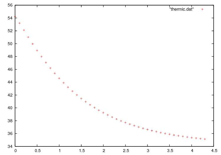
    ff << u(3., 0.5) << endl;
    plot(u);
}

Note

We must separate by hand the bilinear part from the linear one.

Note

The way we store the temperature at point (3, 0.5) for all times in file thermic.dat. Should a one dimensional plot be required (you can use gnuplot tools), the same procedure can be used. For instance to print \(x\mapsto \frac{\partial u}{\partial y}(x,0.9)\) one would do:

for(int i = 0; i < 20; i++)
   cout << dy(u)(6.0*i/20.0,0.9) << endl;

Results are shown on Fig. 13 and Fig. 14.

Thermic — Fig. 13 Temperature at \(t=4.9\).

ThermicVST — Fig. 14 Decay of temperature versus time at \(x=3, y=0.5\)

Thermal conduction

Axisymmetry: 3D Rod with circular section

Let us now deal with a cylindrical rod instead of a flat plate. For simplicity we take \(\kappa=1\).

In cylindrical coordinates, the Laplace operator becomes (\(r\) is the distance to the axis, \(z\) is the distance along the axis, \(\theta\) polar angle in a fixed plane perpendicular to the axis):

\[\Delta u = {1\over r}\partial _r(r\partial _r u) + {1\over r^2}\partial ^2_{\theta\theta} u + \partial ^2_{z z}.\]

Symmetry implies that we loose the dependence with respect to \(\theta\); so the domain \(\Omega\) is again a rectangle \(]0,R[\times]0,|[\) . We take the convention of numbering of the edges as in square() (1 for the bottom horizontal …); the problem is now:

\[\begin{split}\begin{array}{rcl} r\partial_t u-\partial _r(r\partial _r u) - \partial _z(r\partial _z u) &= 0 &\hbox{ in } \Omega\\ u(t=0) &= u_0 + \frac z{L_z} (u_1-u)&\\ u|_{\Gamma_4} &= u_0&\\ u|_{\Gamma_2} &= u_1&\\ \alpha(u-u_e) + {\partial u\over \partial\boldsymbol{n}} |_{\Gamma_1\cup\Gamma_3} &= 0& \end{array}\end{split}\]

Note that the PDE has been multiplied by \(r\).

After discretization in time with an implicit scheme, with time steps dt, in the FreeFEM syntax \(r\) becomes \(x\) and \(z\) becomes \(y\) and the problem is:

problem thermaxi(u, v)
    = int2d(Th)(
          (u*v/dt + dx(u)*dx(v) + dy(u)*dy(v))*x
    )
    + int1d(Th, 3)(
          alpha*x*u*v
    )
    - int1d(Th, 3)(
          alpha*x*ue*v
    )
    - int2d(Th)(
          uold*v*x/dt
    )
    + on(2, 4, u=u0);

Note

The bilinear form degenerates at \(x=0\). Still one can prove existence and uniqueness for \(u\) and because of this degeneracy no boundary conditions need to be imposed on \(\Gamma_1\).

A Nonlinear Problem : Radiation

Heat loss through radiation is a loss proportional to the absolute temperature to the fourth power (Stefan’s Law). This adds to the loss by convection and gives the following boundary condition:

\[\kappa{\partial u\over \partial\boldsymbol{n}} +\alpha(u-u_e) + c[(u + 273)^4 - (u_e+273)^4] = 0\]

The problem is nonlinear, and must be solved iteratively with fixed-point iteration where \(m\) denotes the iteration index, a semi-linearization of the radiation condition gives

\[{\partial u^{m+1}\over \partial\boldsymbol{n}} + \alpha(u^{m+1}-u_e)+ c(u^{m+1}-u_e) (u^m+u_e +546) ((u^m + 273)^2 + (u_e+273)^2) = 0,\]

because we have the identity \(a^4 - b^4 = (a-b)(a+b)(a^2+b^2)\).

The iterative process will work with \(v=u-u_e\).

...
// Mesh
fespace Vh(Th, P1);
Vh vold, w, v=u0-ue, b,vp;

// Problem
problem thermradia(v, w)
    = int2d(Th)(
          v*w/dt
        + k*(dx(v) * dx(w) + dy(v) * dy(w))
    )
    + int1d(Th, 1, 3)(
          b*v*w
    )
    - int2d(Th)(
          vold*w/dt
    )
    + on(2, 4, v=u0-ue)
    ;

verbosity=0; // to remove spurious FREEfem print
for (real t=0;t<T;t+=dt){
  vold[] = v[];// just copy DoF's, faster than interpolation pv=v;
  for (int m = 0; m < 5; m++) {
    vp[]=v[];// save previous state of commute error
    b = alpha + rad * (v + 2*uek) * ((v+uek)^2 + uek^2);
    thermradia;
    vp[]-=v[];
    real err = vp[].linfty;// error value
    cout << " time " << t << " iter " << m << " err = "<< vp[].linfty << endl;
    if( err < 1e-5) break; // if error is enough  small break fixed-point loop
    }
  }
v[] += ue;//  add a constant to all DoF's of v

plot(v);

Here you can use the search bar to search in all FreeFEM examples instead

The list of all matching examples on the right is updated for each new query

Clicking on a search hit or on an example on the right brings up the corresponding script from GitHub

You can also filter the list on the right by selecting one or more intersecting categories on the left tree

Thermal Conduction

Axisymmetry: 3D Rod with circular section

A Nonlinear Problem : Radiation