Finite element
As stated in tutorials, FEM approximates all functions \(w\) as:
with finite element basis functions \(\phi_k(x,y)\) and numbers \(w_k\) (\(k=0,\cdots,M-1\)). The functions \(\phi_k(x,y)\) are constructed from the triangle \(T_{i_k}\), and called shape functions.
In FreeFEM, the finite element space:
is easily created by
in 2d
1fespace IDspace(IDmesh,<IDFE>);or with \(\ell\) pairs of periodic boundary conditions in 2D:
1fespace IDspace(IDmesh,<IDFE>,
2    periodic=[[la1, sa1], [lb1, sb1],
3              ...
4              [lak, sak], [lbk, sbl]]);
in 3D:
1fespace IDspace(IDmesh3,<IDFE>,
2    periodic=[[la1, sa1, ta1], [lb1, sb1, tb1],
3              ...
4              [lak, sak, tak], [lbk, sbl, tbl]]);
in surface 3D:
1fespace IDspace(IDmeshS,<IDFE>,
2    periodic=[[la1, sa1, ta1], [lb1, sb1, tb1],
3              ...
4              [lak, sak, tak], [lbk, sbl, tbl]]);
where IDspace is the name of the space (e.g. Vh), IDmesh IDmesh3 IDmeshS `is respectly the name of the associated :freefem:`mesh, mesh3, meshS and <IDFE> is an identifier of finite element type.
In 2D we have a pair of periodic boundary conditions, if \([la_i, sa_i]\), \([lb_i, sb_i]\) is a pair of int, and the 2 labels \(la_i\) and \(lb_i\) refer to 2 pieces of boundary to be in equivalence.
If \([la_i, sa_i]\), \([lb_i, sb_i]\) is a pair of real, then \(sa_i\) and \(sb_i\) give two common abscissa on the two boundary curves, and two points are identified as one if the two abscissa are equal.
In 2D, we have a pair of periodic boundary conditions, if \([la_i, sa_i, ta_i]\), \([lb_i, sb_i, tb_i]\) is a pair of int, the 2 labels \(la_i\) and \(lb_i\) define the 2 pieces of boundary to be in equivalence.
If \([la_i, sa_i, ta_i]\), \([lb_i, sb_i, tb_i]\) is a pair of real, then \(sa_i\), \(ta_i\) and \(sb_i\), \(tb_i\) give two common parameters on the two boundary surfaces, and two points are identified as one if the two parameters are equal.
Note
The 2D mesh of the two identified borders must be the same, so to be sure, use the parameter fixedborder=true in buildmesh command (see fixedborder).
List of the types of finite elements
As of today, the known types of finite elements are:
[P0]piecewise constant discontinuous finite element (2d, 3d, surface 3d), the degrees of freedom are the barycenter element value.[P1]piecewise linear continuous finite element (2d, 3d, surface 3d), the degrees of freedom are the vertices values.[P1dc]piecewise linear discontinuous finite element (2d, 3d with load”Element_P1dc1”)Warning
Due to an interpolation problem, the degree of freedom is not the vertices but three vertices which move inside \(T(X)= G + .99 (X-G)\) where \(G\) is the barycenter.
[P1b]piecewise linear continuous finite element plus bubble (2d, 3d)The 2D Case:
The 3D Case:
(13)\[\P^1_{b|h} = \left\{ v \in H^{1}(\Omega) \left|\; \forall K \in \mathcal{T}_{h}, \ v_{|K} \in P_{1} \oplus \mathrm{Span}\{ \lambda^{K}_{0} \lambda^{K}_{1} \lambda^{K}_{2} \lambda^{K}_{3} \} \right.\right\}\]where \(\lambda^{K}_{i}, i=0,..,d\) are the \(d+1\) barycentric coordinate functions of the element \(K\) (triangle or tetrahedron).
P1bl,P1bl3dpiecewise linear continuous finite element plus linear bubble (with load”Element_P1bl” 2d, 3d).The bubble is built by splitting the \(K\), a barycenter in \(d+1\) sub element. (need
load "Element_P1bl")[P2, P2]piecewise \(P_{2}\) continuous finite element (2d, 3d, surface 3d)\[\P^2_{h} = \left\{ v \in H^{1}(\Omega) \left|\; \forall K \in \mathcal{T}_{h}, \ v_{|K} \in P_{2} \right.\right\}\]where \(P_{2}\) is the set of polynomials of \(\R^{2}\) of degrees \(\le 2\).
[P2b, P2b3d]piecewise \(P_{2}\) continuous finite element plus bubble (2d, 3d with load”Element_P2bulle3”)The 2D Case:
\[\P^2_{h} = \left\{ v \in H^{1}(\Omega) \left|\; \forall K \in \mathcal{T}_{h}, \ v_{|K} \in P_{2} \oplus \mathrm{Span}\{ \lambda^{K}_{0} \lambda^{K}_{1} \lambda^{K}_{2} \} \right.\right\}\]The 3D Case:
\[\P^2_{h} = \left\{ v \in H^{1}(\Omega) \left|\; \forall K \in \mathcal{T}_{h}, \ v_{|K} \in P_{2} \oplus \mathrm{Span}\{ \lambda^{K}_{0} \lambda^{K}_{1} \lambda^{K}_{2} \lambda^{K}_{3} \} \right.\right\}\][P2dc]piecewise \(P_{2}\) discontinuous finite element (2d)\[\P^2_{dc|h} = \left\{ v \in L^{2}(\Omega) \left|\; \forall K \in \mathcal{T}_{h}, \ v_{|K} \in P_{2} \right.\right\}\]Warning
Due to an interpolation problem, the degree of freedom is not the six P2 nodes but six nodes which move inside \(T(X)= G + .99 (X-G)\) where \(G\) is the barycenter.
[P2h]quadratic homogeneous continuous (withoutP1).[P3]piecewise \(P_{3}\) continuous finite element (2d) (needsload "Element_P3")\[\P^3_{h} = \left\{ v \in H^{1}(\Omega) \left|\; \forall K \in \mathcal{T}_{h}, \ v_{|K} \in P_{3} \right.\right\}\]where \(P_{3}\) is the set of polynomials of \(\R^{2}\) of degrees \(\le 3\).
[P3dc]piecewise \(P_{3}\) discontinuous finite element (2d) (needsload "Element_P3dc")\[\P^3_{dc|h} = \left\{ v \in L^2(\Omega) \left|\; \forall K \in \mathcal{T}_{h}, \ v_{|K} \in P_{3} \right.\right\}\]where \(P_{3}\) is the set of polynomials of \(\R^{2}\) of degrees \(\le 3\).
[P4]piecewise \(P_{4}\) continuous finite element (2d) (needsload "Element_P4")\[\P^4_{h} = \left\{ v \in H^{1}(\Omega) \left|\; \forall K \in \mathcal{T}_{h},\ v_{|K} \in P_{4} \right.\right\}\]where \(P_{4}\) is the set of polynomials of \(\R^{2}\) of degrees \(\le 4\).
[P4dc]piecewise \(P_{4}\) discontinuous finite element (2d) (needsload "Element_P4dc")\[\P^4_{dc|h} = \left\{ v \in L^2(\Omega) \left|\; \forall K \in \mathcal{T}_{h}, \ v_{|K} \in P_{3} \right.\right\}\]where \(P_{4}\) is the set of polynomials of \(\R^{2}\) of degrees \(\le 3\).
[P0Edge]piecewise \(P_{0}\) discontinuous finite element (2d) contained on each edge of the mesh.[P1Edge]piecewise \(P_{1}\) discontinuous finite element (2d) (needsload "Element_PkEdge") \(P_1\) on each edge of the mesh.[P2Edge]piecewise \(P_{2}\) discontinuous finite element (2d) (needsload "Element_PkEdge") \(P_2\) on each edge of the mesh.[P3Edge]piecewise \(P_{3}\) discontinuous finite element (2d) (needsload "Element_PkEdge") \(P_3\) on each edge of the mesh.[P4Edge]piecewise \(P_{4}\) discontinuous finite element (2d) (needsload "Element_PkEdge") \(P_4\) on each edge of the mesh.[P5Edge]piecewise \(P_{5}\) discontinuous finite element (2d) (needsload "Element_PkEdge") \(P_5\) on each edge of the mesh.[P2Morley]piecewise \(P_{2}\) non conform finite element (2d) (needsload "Morley")\[\begin{split}\P^2_{h} = \left\{ v \in L^2(\Omega) \left|\; \forall K \in \mathcal{T}_{h}, \ v_{|K} \in P_{3}, \left\{\begin{array}{c} v \mbox{ continuous at vertices,}\\ \p_n{v} \mbox{ continuous at middle of edge,} \end{array}\right. \right.\right\}\end{split}\]where \(P_{2}\) is the set of polynomials of \(\R^{2}\) of degrees \(\le 2\).
Warning
To build the interplant of a function \(u\) (scalar) for this finite element, we need the function and 2 partial derivatives \((u,u_x, u_y)\), creating this vectorial finite element with 3 components \((u,u_x,u_y)\).
See our example for solving the BiLaplacien problem:
 1load "Morley"
 2
 3// Parameters
 4int nn = 10;
 5real h = 0.01;
 6
 7real f = 1;
 8
 9// Mesh
10mesh Th = square(nn, nn);
11Th = adaptmesh(Th, h, IsMetric=1);
12
13// Fespace
14fespace Vh(Th, P2Morley); //The Morley finite element space
15Vh [u, ux, uy], [v, vx, vy];
16
17// Macro
18macro bilaplacien(u, v) (dxx(u)*dxx(v) + dyy(u)*dyy(v) + 2.*dxy(u)*dxy(v)) //
19
20// Problem
21solve bilap ([u, ux, uy], [v, vx, vy])
22    = int2d(Th)(
23        bilaplacien(u, v)
24    )
25    - int2d(Th)(
26        f*v
27    )
28    + on(1, 2, 3, 4, u=0, ux=0, uy=0)
29    ;
30
31// Plot
32plot(u, cmm="u");
[HCT]\(P_3\) \(C^1\) conforms finite element (2d) (needsload "Element_HCT") one 3 sub triangles.Lets call \(\mathcal{T}^\triangle_{h}\) the sub mesh of \(\mathcal{T}_{h}\) where all triangles are split in 3 at the barycenter.
\[\P^{HCT}_{h} = \left\{ v \in C^1(\Omega) \left|\; \forall K \in \mathcal{T}^\triangle_{h}, \ v_{|K} \in P_{3} \right.\right\}\]where \(P_{3}\) is the set of polynomials of \(\R^{2}\) of degrees \(\le 3\).
The degrees of freedom are the values of the normal derivative at the mid-point of each edge [BERNADOU1980].
Warning
To build the interplant of a function \(u\) (scalar) for this finite element, we need the function and 2 partial derivatives \((u,u_x, u_y)\), creating this vectorial finite element with 3 components \((u,u_x,u_y)\) like in previous finite element.
[P2BR](needsload "BernadiRaugel") the Bernadi Raugel Finite Element is a Vectorial element (2d) with 2 components, see [BERNARDI1985].It is a 2D coupled Finite Element, where the Polynomial space is \(P_1^2\) with 3 normal bubble edge functions \((P_2)\). There are 9 degrees of freedom:
2 components at each of the 3 vertices and
the 3 flux on the 3 edges.
[RT0, RT03d]Raviart-Thomas finite element of degree \(0\).The 2D Case:
(14)\[RT0_{h} = \left\{ \mathbf{v} \in H(\textrm{div}) \left|\; \forall K \in \mathcal{T}_{h} ,\ \mathbf{v}_{|K}(x,y) = \vecttwo{\alpha^1_{K}}{\alpha^2_{K}} + \beta_{K}\vecttwo{x}{y} \right.\right\}\]The 3D Case:
(15)\[RT0_{h} = \left\{ \mathbf{v} \in H(\textrm{div}) \left|\; \forall K \in \mathcal{T}_{h},\ \mathbf{v}_{|K}(x,y,z) = \vectthree{\alpha^1_{K}}{\alpha^2_{K}}{\alpha^3_{K}} + \beta_{K}\vectthree{x}{y}{z} \right.\right\}\]where by writing \(\textrm{div }\mathbf{w}=\sum_{i=1}^d\p w_i/\p x_i\) with \(\mathbf{w}=(w_i)_{i=1}^d\):
\[H(\textrm{div})=\left\{\mathbf{w}\in L^{2}(\Omega)^d\left|\textrm{div } \mathbf{w}\in L^{2}(\Omega)\right.\right\}\]and where \(\alpha^1_{K}\), \(\alpha^2_{K}\), \(\alpha^3_{K}\), \(\beta_{K}\) are real numbers.
[RT0Ortho]Raviart-Thomas Orthogonal, or Nedelec finite element type I of degree \(0\) in dimension 2[Edge03d]3d Nedelec finite element or Edge Element of degree \(0\).\[Edge0_{h} = \left\{ \mathbf{v} \in H(\textrm{Curl}) \left|\; \forall K \in\mathcal{T}_{h}, \ \mathbf{v}_{|K}(x,y,z) = \vectthree{\alpha^1_{K}}{\alpha^2_{K}}{\alpha^3_{K}} + \vectthree{\beta^1_{K}}{\beta^2_{K}}{\beta^3_{K}}\times\vectthree{x}{y}{z} \right.\right\} :label:eq:Edge03d\]where by writing \(\textrm{curl}\mathbf{w}=\vectthree{\p w_2/\p x_3-\p w_3/\p x_2}{\p w_3/\p x_1-\p w_1/\p x_3}{\p w_1/\p x_2-\p w_2/\p x_1}\) with \(\mathbf{w}=(w_i)_{i=1}^d\):
\[H(\textrm{curl})=\left\{\mathbf{w}\in L^{2}(\Omega)^d\left|\textrm{curl } \mathbf{w}\in L^{2}(\Omega)^d\right.\right\}\]and \(\alpha^1_{K},\alpha^2_{K},\alpha^3_{K},\beta^1_{K},\beta^2_{K},\beta^3_{K}\) are real numbers.
[Edge13d](needsload "Element_Mixte3d") 3d Nedelec finite element or Edge Element of degree \(1\).[Edge23d](needsload "Element_Mixte3d") 3d Nedelec finite element or Edge Element of degree \(2\).[P1nc]piecewise linear element continuous at the mid-point of the edge only in 2D (Crouzeix-Raviart Finite Element 2D).[P2pnc]piecewise quadratic plus a P3 bubble element with the continuity of the 2 moments on each edge (needsload "Element_P2pnc")[RT1](needsload "Element_Mixte")[RT1Ortho](needsload "Element_Mixte")[RT2](needsload "Element_Mixte")[RT2Ortho](needsload "Element_Mixte")[BDM1](needsload "Element_Mixte") the Brezzi-Douglas-Marini finite element:[BDM1Ortho](needsload "Element_Mixte") the Brezzi-Douglas-Marini Orthogonal also call Nedelec of type II , finite element[FEQF](needsload "Element_QF") the finite element to store functions at default quadrature points (so the quadrature isqf5pTin 2D and isqfV5in 3d).For over quadrature you have the following corresponding finite element’s quadrature formula.
FEQF1\(\mapsto\)qf1pT,FEQF2\(\mapsto\)qf2pT,FEQF5\(\mapsto\)qf5pT,FEQF7\(\mapsto\)qf7pT,FEQF9\(\mapsto\)qf9pT,FEQF13d\(\mapsto\)qfV1,FEQF23d\(\mapsto\)qfV2,FEQF53d\(\mapsto\)qfV5
You can use this element to optimize the storage and reuse of functions with a long formula inside an integral for non linear processes.
Use of fespace in 2D
With the 2D finite element spaces
when \(\mathcal{T}_h\) is a mesh \(10\times 10\) of the unit square \(]0,1[^2\), we only write in FreeFEM:
1mesh Th = square(10, 10);
2fespace Xh(Th, P1); //scalar FE
3fespace Xph(Th,P1,
4    periodic=[[2, y], [4, y], [1, x], [3, x]]); //bi-periodic FE
5fespace Mh(Th, P2); //scalar FE
6fespace Rh(Th, RT0); //vectorial FE
where Xh, Mh, Rh expresses finite element spaces (called FE spaces) \(X_h,\, M_h,\, R_h\), respectively.
To use FE-functions \(u_{h},v_{h} \in X_{h}\), \(p_{h},q_{h} \in M_{h}\) and \(U_{h},V_{h} \in R_{h}\), we write:
1Xh uh, vh;
2Xph uph, vph;
3Mh ph, qh;
4Rh [Uxh, Uyh], [Vxh, Vyh];
5Xh[int] Uh(10);         //array of 10 functions in Xh
6Rh[int] [Wxh, Wyh](10); //array of 10 functions in Rh
7Wxh[5](0.5,0.5);        //the 6th function at point (0.5, 0.5)
8Wxh[5][];               //the array of the degree of freedom of the 6th function
The functions \(U_{h}, V_{h}\) have two components so we have
Use of fespace in 3D
With the 3D finite element spaces
when \(\mathcal{T}_h\) is a mesh \(10\times 10\times 10\) of the unit cubic \(]0,1[^2\), we write in FreeFEM:
 1//label: 0 up, 1 down, 2 front, 3 left, 4 back, 5 right
 2    int nn=10;
 3    mesh3 Th=buildlayers(square(nn,nn,region=0),nn,
 4      zbound=[zmin,zmax], labelmid=rmid, reffaceup = rup,
 5      reffacelow = rdown);
 6
 7fespace Xh(Th, P1); //scalar FE
 8    // a FE space with full periodic condition in 3 axes
 9    fespace Xph(Th,P1,periodic=[[1,y,z],[2,y,z],
10                     [3,x,z],[4,x,z],[5,x,y],[6,x,y]]);
11fespace Mh(Th, P2); //scalar FE
12fespace Rh(Th, RT03d); //vectorial FE
where Xh, Mh, Rh expresses finite element spaces (called FE spaces) \(X_h,\, M_h,\, R_h\), respectively.
The functions \(U_{h}, V_{h}\) have two components so we have
Use of fespace in surface 3D
With the 3D finite element spaces
1meshS Th = square3(10, 10);
2fespace Xh(Th, P1); //scalar FE
where Xh expresses finite element spaces (called FE spaces) \(X_h\), respectively.
To use FE-functions \(u_{h},v_{h} \in X_{h}\), \(p_{h},q_{h} \in M_{h}\) and \(U_{h},V_{h} \in R_{h}\), we write:
1Xh uh, vh;
2Xh[int] Uh(10);         //array of 10 functions in Xh
Finite Element functions
To define and use FE-functions \(u_{h},v_{h} \in X_{h}\), \(p_{h},q_{h} \in M_{h}\) and \(U_{h},V_{h} \in R_{h}\), we write:
1Xh uh, vh;
2Xph uph, vph;
3Mh ph, qh;
4Rh [Uxh, Uyh, Uyzh], [Vxh, Vyh, Vyzh];
5Xh[int] Uh(10);             //array of 10 functions in Xh
6Rh[int] [Wxh,Wyh,Wzh](10);  // array of 10 functions in Rh
7Wxh[5](0.5,0.5,0.5);        //the 6th function at point (0.5, 0.5, 0.5)
8Wxh[5][];                   //the array of the degree of freedom of the 6th function
The functions \(U_{h}, V_{h}\) have three components, so we have:
Note
One challenge of the periodic boundary condition is that the mesh must have equivalent faces.
The buildlayers mesh generator splits each quadrilateral face with the diagonal passing through the vertex with maximum number, so to be sure to have the same mesh one both face periodic the 2D numbering in corresponding edges must be compatible (for example the same variation).
By Default, the numbering of square vertex is correct.
To change the mesh numbering you can use the change function like:
1{
2    int[int] old2new(0:Th.nv-1); //array set on 0, 1, .., nv-1
3    fespace Vh2(Th, P1);
4    Vh2 sorder = x+y; //choose an order increasing on 4 square borders with x or y
5    sort(sorder[], old2new); //build the inverse permutation
6    int[int] new2old = old2new^-1; //inverse the permutation
7    Th = change(Th, renumv=new2old);
8}
The full example is in examples.
Lagrangian Finite Elements
P0-element
For each triangle (d=2) or tetrahedron (d=3) \(T_k\), the basis function \(\phi_k\) in Vh(Th, P0) is given by:
If we write:
1Vh(Th, P0);
2Vh fh = f(x,y);
then for vertices \(q^{k_i},\, i=1,2,.. d+1\) in Fig. 98, \(f_h\) is built as fh= \(\displaystyle f_h(x,y)=\sum_k f(\frac{\sum_i q^{k_i}}{d+1}) \phi_k\)
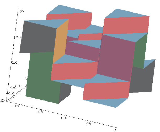
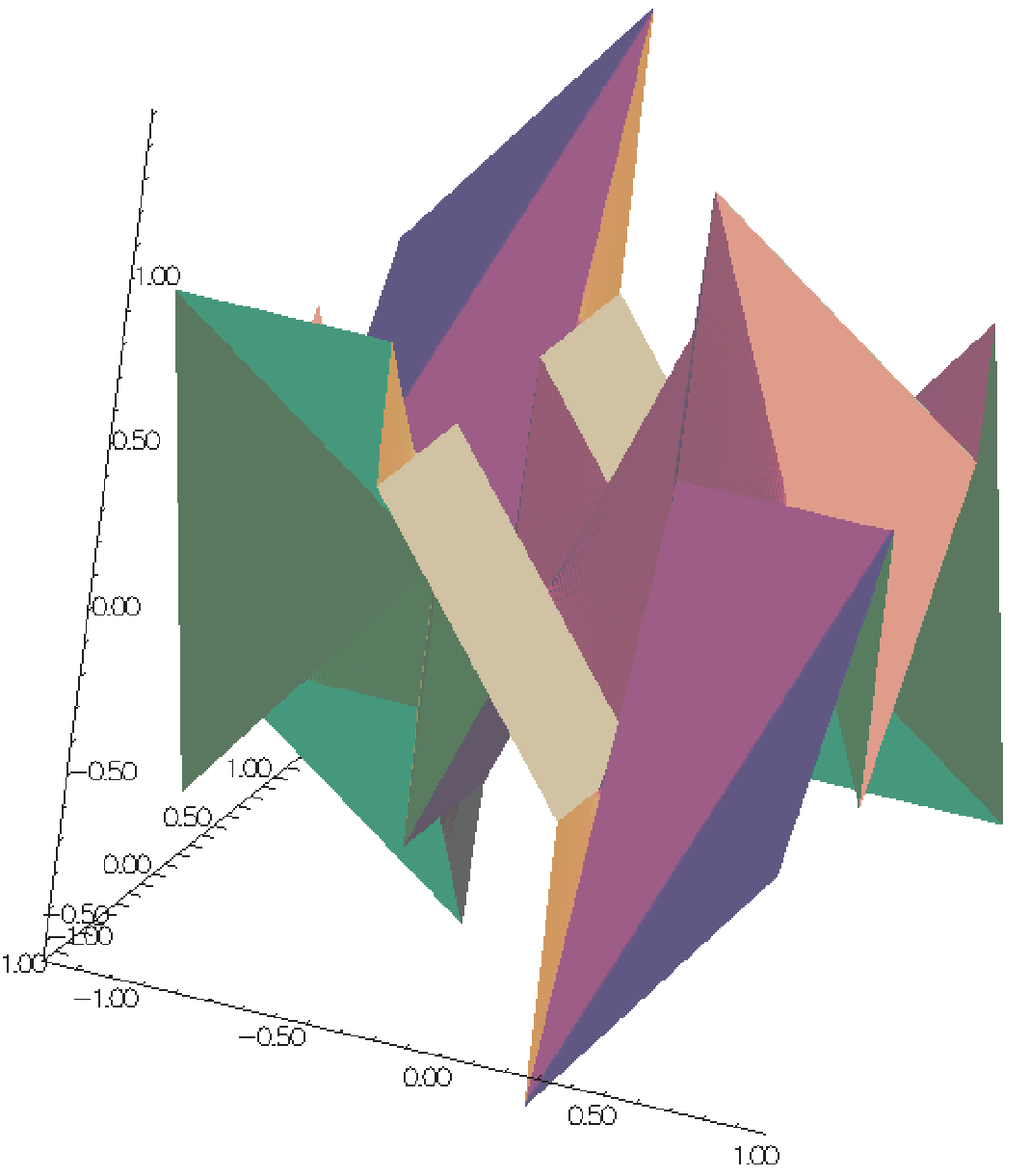
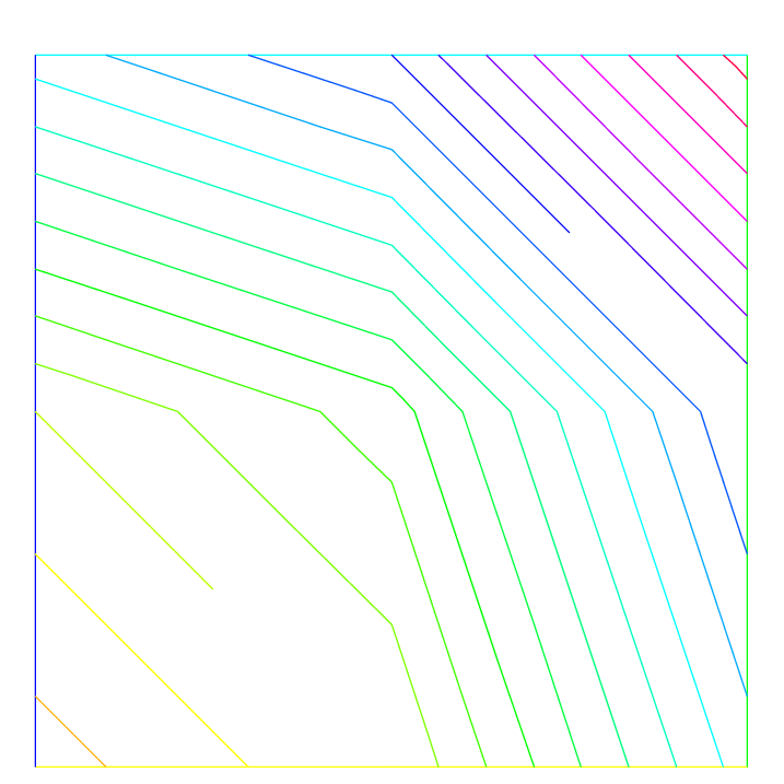
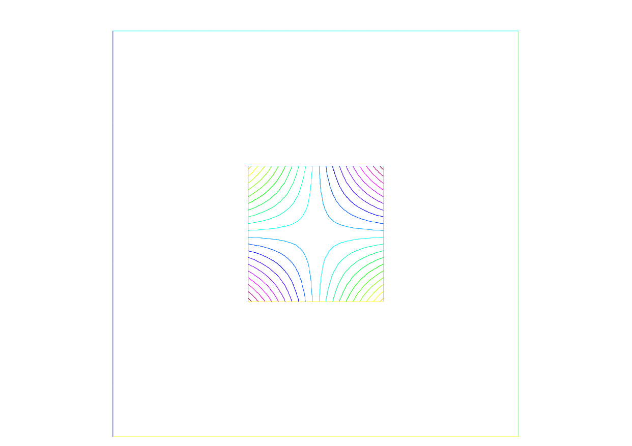
See Fig. 100 for the projection of \(f(x,y)=\sin(\pi x)\cos(\pi y)\) on Vh(Th, P0) when the mesh Th is a \(4\times 4\)-grid of \([-1,1]^2\) as in Fig. 99.
P1-element
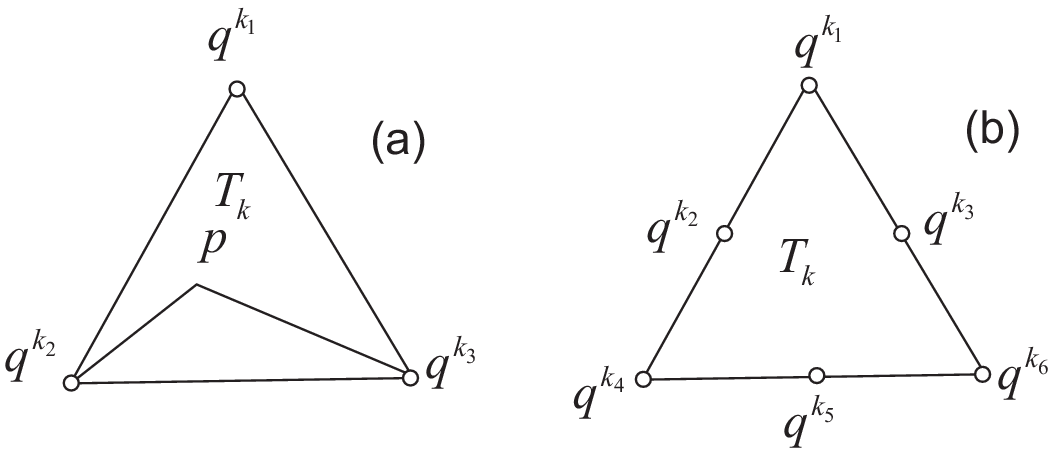
Fig. 98 \(P_1\) and \(P_2\) degrees of freedom on triangle \(T_k\)
For each vertex \(q^i\), the basis function \(\phi_i\) in Vh(Th, P1) is given by:
The basis function \(\phi_{k_1}(x,y)\) with the vertex \(q^{k_1}\) in Fig. 98 at point \(p=(x,y)\) in triangle \(T_k\) simply coincide with the barycentric coordinates \(\lambda^k_1\) (area coordinates):
If we write:
1Vh(Th, P1);
2Vh fh = g(x.y);
then:
fh = \(\displaystyle f_h(x,y)=\sum_{i=1}^{n_v}f(q^i)\phi_i(x,y)\)
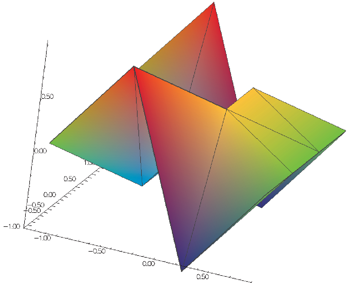
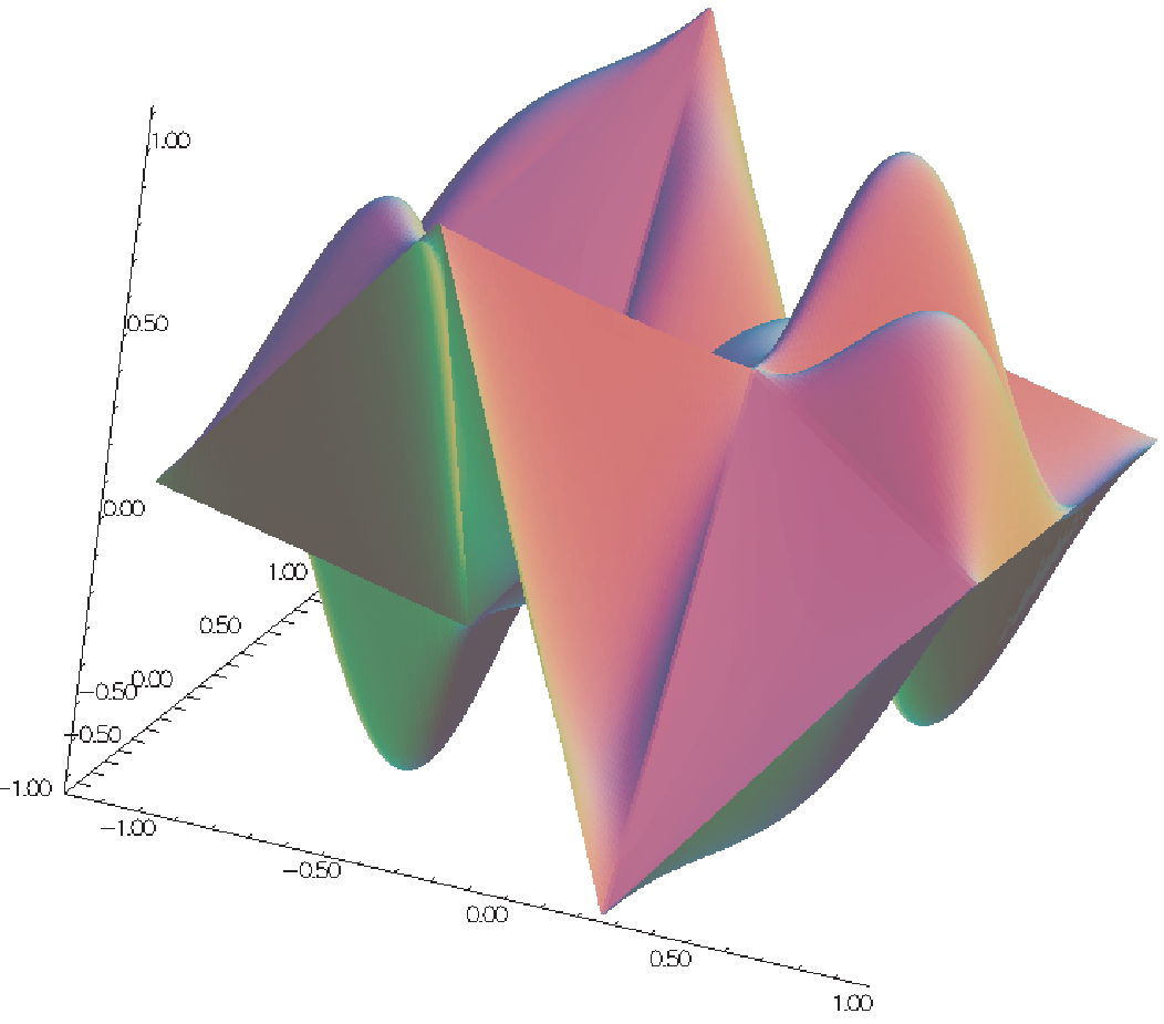
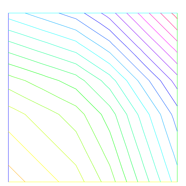
See Fig. 101 for the projection of \(f(x,y)=\sin(\pi x)\cos(\pi y)\) into Vh(Th, P1).

P2-element
For each vertex or mid-point \(q^i\).
The basis function \(\phi_i\) in Vh(Th, P2) is given by:
The basis function \(\phi_{k_1}(x,y)\) with the vertex \(q^{k_1}\) in Fig. 98 is defined by the barycentric coordinates:
and for the mid-point \(q^{k_2}\):
If we write:
1Vh(Th, P2);
2Vh fh = f(x.y);
then:
fh = \(\displaystyle f_h(x,y)=\sum_{i=1}^{M}f(q^i)\phi_i(x,y)\quad (\textrm{summation over all vertex or mid-point})\)
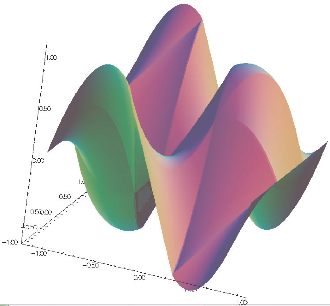
See Projection to Vh(Th, P2) for the projection of \(f(x,y)=\sin(\pi x)\cos(\pi y)\) into Vh(Th, P2).
Surface Lagrangian Finite Elements
Definition of the surface P1 Lagragian element
To build the surface Pk-Lagrange, the main idea is to consider the usual 2d Lagrangian Finite Elements ; and its writing in barycentric coordinates ; apply a space transformation and barycentric properties.
The FreeFEM finite elements for surface problem are: P0 P1 P2 P1b.
0) Notation
Let \(\hat K\) be the shape triangle in the space \(\mathbb{R}^2\) of vertice \((i_0,i_1,i_2)\)
Let \(K\) be a triangle of the space \(\mathbb{R}^3\) of vertice \((A_0,A_1,A_2)\)
\(x_q\) a quadrature point on K
\(X_q\) a quadrature point on A
\(P1_{2d}\) designates 2d P1 Lagrangian Finite Elements
\(P1_{S}\) designates surface 3d P1 Lagrangian Finite Elements
\((\lambda_i)_{i=0}^2\) shape fonction of \(\hat K\) (\(P1_{2d}\))
\((\psi_i)_{i=0}^2\) shape fonction of of \(K\) (\(P1_S\) )
1) Geometric transformation: from the current FE to the reference FE
Let be \(\hat x= \begin{pmatrix} \hat x \\ \hat y \end{pmatrix}\) a point of the triangle \(\hat K \subset \mathbb{R}^2\) and \(X= \begin{pmatrix} x \\ y \\ z \end{pmatrix}\) a point of the triangle \(K \subset \mathbb{R}^3\), where \(\hat x\) and \(\hat X\) are expressed in baricentric coordinates.
The motivation here is to parameterize the 3d surface mesh to the reference 2d triangle, thus to be reduced to a finite element 2d P1. Let’s define a geometric transformation F, such as \(F: \mathbb{R}^2 \rightarrow \mathbb{R}^3\)
However, thus defines transformation F as not bijective.
So, consider the following approximation
where \(\wedge\) denote the usual vector product.
Fig. 103 F, a parameterization from the reference 2d triangle to a 3d surface triangle
Note
\(\overrightarrow {A0A1} \wedge \overrightarrow {A_0A_2} = \begin{pmatrix} n_x \\ n_y \\ n_z \end{pmatrix}\) defines the normal to the tangent plane generated by \(( A_0,\overrightarrow {A_0A_1}, \overrightarrow {A_0A_2} )\)
The affine transformation \(\tilde F\) allows you to pass from the 2d reference triangle, which we project in \(\mathbb{R}^3\) to the 3d current triangle, discretizing the surface we note \(\Gamma\).
Then \(\tilde F^{-1}\) is well defined and allows to return to the reference triangle \(\hat K\), to the usual coordinates of \(\mathbb{R}^2\) completed by the coordinate \(z=0\).
2) Interpolation element fini
Remember that the reference geometric element for the finite element \(P1s\) that we are building is the reference triangle \(\hat K\) in the vertex plane \((i_0, i_1, i_2\)), which we project into space by posing \(z=0\) by the membrane hypothesis.
Hence \(i_0 = \begin{pmatrix} 0 \\ 0 \\ 0 \end{pmatrix}\), \(i_1 = \begin{pmatrix} 1 \\ 0 \\ 0 \end{pmatrix}\), \(i_1 = \begin{pmatrix} 0 \\ 1 \\ 0 \end{pmatrix}\).
Let X be a point of the current triangle K, we have X= \(\tilde F(\hat{x})\). The barycentric coordinates of X in K are given by: \(X = \sum_{i=0} ^2 A_i \hat \lambda(\hat{x})\) où
\(A_i\) the points of the current triangle K
\(\hat \lambda_i\) basic functions \(P1_{2d}\)
\(\hat \lambda_0(x,y) = 1-x-y\)
\(\hat \lambda_1(x,y) = x\)
\(\hat \lambda_2(x,y) = y\)
We need to define a quadrature formula for the finite element approximation. The usual formulation for a 2d triangle will be used by redefining the quadrature points \(X_q = x_q = \begin{pmatrix} \hat x_q \\ \hat y_q \\ 0 \end{pmatrix}\).
3) The Lagragian P1 functions and theirs 1st order derivatives
The finite element interpolation gives us the following relationship: \(\psi_i(X) = F^{-1} (\psi_i)( F^{-1} (X))\). To find the expression of the basic functions \(\psi\) on the current triangle K, it is sufficient to use the inverse of the transformation \(\tilde F\) to get back to the reference triangle \(\hat K\). However in FreeFEM, the definition of the reference finite element, the current geometry is based on barycentric coordinates in order not to use geometric transformation. \(\tilde F\). The method used here is geometric and based on the properties of the vector product and the area of the current triangle K.
i) The shape functions
Let be the triangle K of vertices \(i_0, i_1, i_2 \subset \mathbb{R}^3\) and \((\lambda_i)_{i=0} ^2\) the local barycentric coordinates at K. The normal is defined as the tangent plane generated by \((A_0, \overrightarrow {A_0A_1}, \overrightarrow {A_0A_2})\), \ \(\vec n = \overrightarrow {A_0A_1} \wedge \overrightarrow {A_0A_2}\) avec \(\mid \mid \vec n \mid \mid = 2 \text{ mes }(\hat K)\).
Le denotes the operator V, defines the usual vector product of \(\mathbb{R}^3\) such as \(V(A,B,C) = (B-A) \wedge (C-A)\)
The mixed product of three vectors u, v, w, noté \([u, v, w]\), is the determinant of these three vectors in any direct orthonormal basis, thus \((A \wedge V,C)= \text{ det }(A,B,C)\)
with \((.,.)\) is the usual scalar product of \(\mathbb{R}^3\). \ Let Ph :math:` in mathbb{R}^3` and P his projected in the triangle K such as:
Let’s lay the sub-triangles as follows :
\(K_0 = (P,A1,A2)\)
\(K_1 = (A0,P,A2)\)
\(K_2 = (A0,A1,P)\)
with \(K = K_0 \cup K_1 \cup K_2\).
Note
- Properties in \(\mathbb{R}^3\)
Let \(\vec n\) be the normal to the tangent plane generated by \((A_0, \overrightarrow {A_0A_1}, \overrightarrow {A_0A_2})\)
\(\vec n =\overrightarrow {A_0 A_1} \wedge \overrightarrow {A_0 A_2}\)
By definition, \(\mathcal{A}= \frac{1}{2} \mid < \vec n,\vec n> \mid\) and the vectorial area by \(\mathcal{A^S}= \frac{1}{2} < \vec n,\vec n>\) hence \(\mathcal{A^S} (PBC)= \frac{1}{2} < \vec n_0,\vec n>\), with \(\vec n_0\) the normal vector to the plane (PBC)
Let’s define the respective vector areas
\(\vec N_0(P) = V(P,A1,A2)\) the vectorial area of K0
\(\vec N_1(P) = V(A0,P,A2)\) the vectorial area of K1
\(\vec N_2(P) = V(A0,A1,P)\) the vectorial area of K2
By definition, in 3d, the barycentric coordinates are given by algebraic area ratio: :math:` lambda_i(P) = frac {(vec N_i(P),vec N)}{(vec N,vec N)}label{basisfunc}`
Note that \((\vec N_i(P) ,\vec N) = 2 \text{ sign } \text{ mes } (K_i) \mid \mid \vec N \mid \mid\) and \((\vec N,\vec N) = 2 \text{ sign } \text{ mes } (K) \mid \mid \vec N \mid \mid\), avec \(sign\) the orientation of the current triangle compared to the reference triangle.
We find the finite element interpolation, \(P = \sum_{i=0}^2 \lambda_i(P) A_i\).
ii) 1st order derivatives of Lagrangian P1 FE
Let \(\vec Y\) be any vector of \(\in \mathbb{R}^3\).
Let’s calculate the differential of \((\vec N_2(P),Y), \forall Y\)
Consider in particular \(\vec Y = \vec N\), then
This leads to :math:` nabla_P lambda_2(P) = frac {(vec N wedge E_2)}{(vec N,vec N)} `
By similar calculations for \(\vec N_0(P)$ et $\vec N_1(P)\)
\(\nabla_P \lambda_i(P) = \frac {(\vec N \wedge E_i)}{(\vec N,\vec N)}\label{derivbasisfunc}\)
Note
With the definition of the surface gradient and the 2d Pk-Lagrange FE used barycentric coordinates, surface Pk-Langrange FE are trivial.
P1 Nonconforming Element
Refer to [THOMASSET2012] for details; briefly, we now consider non-continuous approximations so we will lose the property:
If we write:
1Vh(Th, P1nc);
2Vh fh = f(x.y);
then:
fh = \(\displaystyle f_h(x,y)=\sum_{i=1}^{n_v}f(m^i)\phi_i(x,y)\quad (\textrm{summation over all midpoint})\)
Here the basis function \(\phi_i\) associated with the mid-point \(m^i=(q^{k_i}+q^{k_{i+1}})/2\) where \(q^{k_i}\) is the \(i\)-th point in \(T_k\), and we assume that \(j+1=0\) if \(j=3\):
Strictly speaking \(\p \phi_i/\p x,\, \p \phi_i/\p y\) contain Dirac distribution \(\rho \delta_{\p T_k}\).
The numerical calculations will automatically ignore them. In [THOMASSET2012], there is a proof of the estimation
The basis functions \(\phi_k\) have the following properties.
For the bilinear form \(a\) defined in Fig. 104 satisfy:
\[\begin{split}\begin{array}{rcl} a(\phi_i,\phi_i)>0,\qquad a(\phi_i,\phi_j)&\le& 0\quad\textrm{if }i\neq j\\ \sum_{k=1}^{n_v}a(\phi_i,\phi_k)&\ge& 0 \end{array}\end{split}\]\(f\ge 0 \Rightarrow u_h\ge 0\)
If \(i\neq j\), the basis function \(\phi_i\) and \(\phi_j\) are \(L^2\)-orthogonal:
\[\int_{\Omega}\phi_i\phi_j\, \d x\d y=0\qquad \textrm{if }i\neq j\]which is false for \(P_1\)-element.
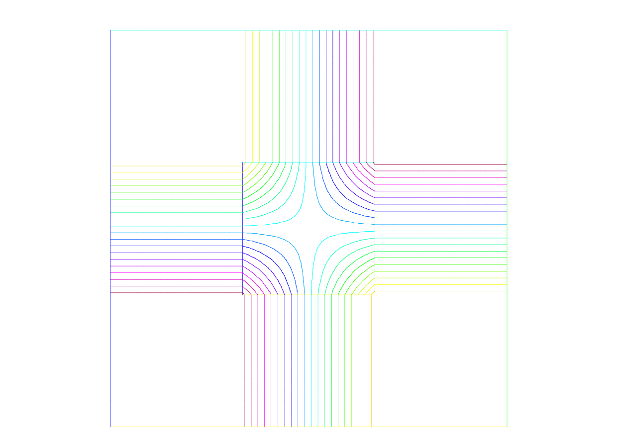
See Fig. 104 for the projection of \(f(x,y)=\sin(\pi x)\cos(\pi y)\) into Vh(Th, P1nc).
Other FE-space
For each triangle \(T_k\in \mathcal{T}_h\), let \(\lambda_{k_1}(x,y),\, \lambda_{k_2}(x,y),\, \lambda_{k_3}(x,y)\) be the area cordinate of the triangle (see Fig. 98), and put:
called bubble function on \(T_k\). The bubble function has the feature: 1. \(\beta_k(x,y)=0\quad \textrm{if }(x,y)\in \p T_k\).
\(\beta_k(q^{k_b})=1\) where \(q^{k_b}\) is the barycenter \(\frac{q^{k_1}+q^{k_2}+q^{k_3}}{3}\).
If we write:
1Vh(Th, P1b);
2Vh fh = f(x.y);
then:
fh = \(\displaystyle f_h(x,y)=\sum_{i=1}^{n_v}f(q^i)\phi_i(x,y)+\sum_{k=1}^{n_t}f(q^{k_b})\beta_k(x,y)\)
See Fig. 105 for the projection of \(f(x,y)=\sin(\pi x)\cos(\pi y)\) into Vh(Th, P1b).
Vector Valued FE-function
Functions from \(\R^{2}\) to \(\R^{N}\) with \(N=1\) are called scalar functions and called vector valued when \(N>1\). When \(N=2\)
1fespace Vh(Th, [P0, P1]) ;
makes the space
Raviart-Thomas Element
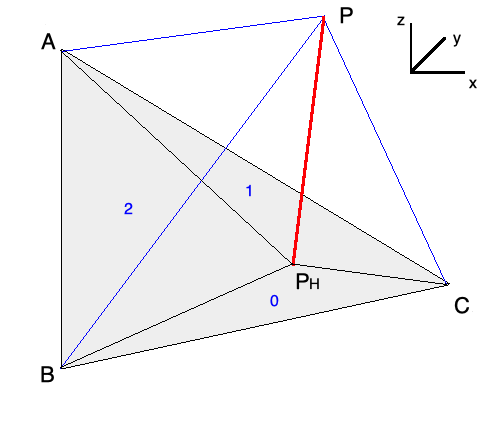
In the Raviart-Thomas finite element \(RT0_{h}\), the degrees of freedom are the fluxes across edges \(e\) of the mesh, where the flux of the function \(\mathbf{f} : \R^2 \longrightarrow \R^2\) is \(\int_{e} \mathbf{f}.n_{e}\), \(n_{e}\) is the unit normal of edge \(e\).
This implies an orientation of all the edges of the mesh, for example we can use the global numbering of the edge vertices and we just go from small to large numbers.
To compute the flux, we use a quadrature with one Gauss point, the mid-point of the edge.
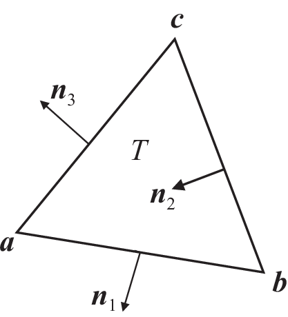
Consider a triangle \(T_k\) with three vertices \((\mathbf{a},\mathbf{b},\mathbf{c})\).
Lets denote the vertices numbers by \(i_{a},i_{b},i_{c}\), and define the three edge vectors \(\mathbf{e}^{1},\mathbf{e}^{2},\mathbf{e}^{3}\) by \(sgn(i_{b}-i_{c})(\mathbf{b}-\mathbf{c})\), \(sgn(i_{c}-i_{a})(\mathbf{c}-\mathbf{a})\), \(sgn(i_{a}-i_{b})(\mathbf{a}-\mathbf{b})\).
We get three basis functions:
where \(|T_k|\) is the area of the triangle \(T_k\). If we write:
1Vh(Th, RT0);
2Vh [f1h, f2h] = [f1(x, y), f2(x, y)];
then:
fh = \(\displaystyle \mathbf{f}_h(x,y)=\sum_{k=1}^{n_t}\sum_{l=1}^6 n_{i_lj_l}|\mathbf{e^{i_l}}|f_{j_l}(m^{i_l})\phi_{i_lj_l}\)
where \(n_{i_lj_l}\) is the \(j_l\)-th component of the normal vector \(\mathbf{n}_{i_l}\),
and \(i_l=\{1,1,2,2,3,3\},\, j_l=\{1,2,1,2,1,2\}\) with the order of \(l\).
 1// Mesh
 2mesh Th = square(2, 2);
 3
 4// Fespace
 5fespace Xh(Th, P1);
 6Xh uh = x^2 + y^2, vh;
 7
 8fespace Vh(Th, RT0);
 9Vh [Uxh, Uyh] = [sin(x), cos(y)]; //vectorial FE function
10
11// Change the mesh
12Th = square(5,5);
13
14//Xh is unchanged
15//Uxh = x; //error: impossible to set only 1 component
16          //of a vector FE function
17vh = Uxh;//ok
18//and now vh use the 5x5 mesh
19//but the fespace of vh is always the 2x2 mesh
20
21// Plot
22plot(uh);
23uh = uh; //do a interpolation of uh (old) of 5x5 mesh
24        //to get the new uh on 10x10 mesh
25plot(uh);
26
27vh([x-1/2, y]) = x^2 + y^2; //interpolate vh = ((x-1/2)^2 + y^2)
To get the value at a point \(x=1,y=2\) of the FE function uh, or [Uxh, Uyh], one writes:
1real value;
2value = uh(2,4); //get value = uh(2, 4)
3value = Uxh(2, 4); //get value = Uxh(2, 4)
4//OR
5x = 1; y = 2;
6value = uh; //get value = uh(1, 2)
7value = Uxh; //get value = Uxh(1, 2)
8value = Uyh; //get value = Uyh(1, 2)
To get the value of the array associated to the FE function uh, one writes
1real value = uh[][0]; //get the value of degree of freedom 0
2real maxdf = uh[].max; //maximum value of degree of freedom
3int size = uh.n; //the number of degree of freedom
4real[int] array(uh.n) = uh[]; //copy the array of the function uh
Warning
For a non-scalar finite element function [Uxh, Uyh] the two arrays Uxh[] and Uyh[] are the same array, because the degree of freedom can touch more than one component.
A Fast Finite Element Interpolator
In practice, one may discretize the variational equations by the Finite Element method. Then there will be one mesh for \(\Omega_1\) and another one for \(\Omega_2\). The computation of integrals of products of functions defined on different meshes is difficult.
Quadrature formula and interpolations from one mesh to another at quadrature points are needed. We present below the interpolation operator which we have used and which is new, to the best of our knowledge.
Let \({\cal T}_{h}^0=\cup_k T^0_k,{\cal T}_{h}^1=\cup_k T^1_k\) be two triangulations of a domain \(\Omega\). Let:
be the spaces of continuous piecewise affine functions on each triangulation.
Let \(f\in V({\cal T}_{h}^0)\). The problem is to find \(g\in V({\cal T}_{h}^1)\) such that:
Although this is a seemingly simple problem, it is difficult to find an efficient algorithm in practice.
We propose an algorithm which is of complexity \(N^1\log N^0\), where \(N^i\) is the number of vertices of \(\cal T_{h}^i\), and which is very fast for most practical 2D applications.
Algorithm
The method has 5 steps.
First a quadtree is built containing all the vertices of the mesh \({\cal T}_{h}^0\) such that in each terminal cell there are at least one, and at most 4, vertices of \({\cal T}_{h}^0\).
For each \(q^1\), vertex of \({\cal T}_{h}^1\) do:
Find the terminal cell of the quadtree containing \(q^1\).
Find the the nearest vertex \(q^0_j\) to \(q^1\) in that cell.
Choose one triangle \(T_k^0\in{\cal T}_{h}^0\) which has \(q^0_j\) for vertex.
Compute the barycentric coordinates \(\{\lambda_j\}_{j=1,2,3}\) of \(q^1\) in \(T^0_k\).
if all barycentric coordinates are positive, go to Step 5
otherwise, if one barycentric coordinate \(\lambda_i\) is negative, replace \(T^0_k\) by the adjacent triangle opposite \(q^0_i\) and go to Step 4.
otherwise, if two barycentric coordinates are negative, take one of the two randomly and replace \(T^0_k\) by the adjacent triangle as above.
Calculate \(g(q^1)\) on \(T^0_k\) by linear interpolation of \(f\):
\[g(q^1) = \sum_{j=1,2,3} \lambda_j f(q^0_j)\]
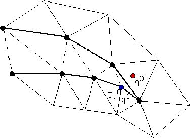
Fig. 109 To interpolate a function at \(q^0\), the knowledge of the triangle which contains \(q^0\) is needed. The algorithm may start at \(q^1\in T_k^0\) and stall on the boundary (thick line) because the line \(q^0q^1\) is not inside \(\Omega\). But if the holes are triangulated too (doted line) then the problem does not arise.
Two problems need to be solved:
What if :math:`q^1` is not in \(\Omega^0_h\) ? Then Step 5 will stop with a boundary triangle.
So we add a step which tests the distance of \(q^1\) with the two adjacent boundary edges and selects the nearest, and so on till the distance grows.
What if \(\Omega^0_h\) is not convex and the marching process of Step 4 locks on a boundary? By construction Delaunay-Voronoï’s mesh generators always triangulate the convex hull of the vertices of the domain.
Therefore, we make sure that this information is not lost when \({\cal T}_{h}^0,{\cal T}_{h}^1\) are constructed and we keep the triangles which are outside the domain on a special list.
That way, in step 5 we can use that list to step over holes if needed.
Note
Sometimes, in rare cases, the interpolation process misses some points, we can change the search algorithm through a global variable searchMethod
1searchMethod = 0; // default value for fast search algorithm
2searchMethod = 1; // safe search algorithm, uses brute force in case of missing point
3// (warning: can be very expensive in cases where a lot of points are outside of the domain)
4searchMethod = 2; // always uses brute force. It is very computationally expensive.
Note
Step 3 requires an array of pointers such that each vertex points to one triangle of the triangulation.
Note
The operator = is the interpolation operator of FreeFEM, the continuous finite functions are extended by continuity to the outside of the domain.
Try the following example :
 1// Mesh
 2mesh Ths = square(10, 10);
 3mesh Thg = square(30, 30, [x*3-1, y*3-1]);
 4plot(Ths, Thg, wait=true);
 5
 6// Fespace
 7fespace Ch(Ths, P2);
 8Ch us = (x-0.5)*(y-0.5);
 9
10fespace Dh(Ths, P2dc);
11Dh vs = (x-0.5)*(y-0.5);
12
13fespace Fh(Thg, P2dc);
14Fh ug=us, vg=vs;
15
16// Plot
17plot(us, ug, wait=true);
18plot(vs, vg, wait=true);
Keywords: Problem and Solve
For FreeFEM, a problem must be given in variational form, so we need a bilinear form \(a(u,v)\), a linear form \(\ell(f,v)\), and possibly a boundary condition form must be added.
1problem P (u, v)
2    = a(u,v) - l(f,v)
3    + (boundary condition)
4    ;
Note
When you want to formulate the problem and solve it in the same time, you can use the keyword solve.
Weak Form and Boundary Condition
To present the principles of Variational Formulations, also called weak form, for the Partial Differential Equations, let’s take a model problem: a Poisson equation with Dirichlet and Robin Boundary condition.
The problem: Find \(u\) a real function defined on a domain \(\Omega\) of \(\R^d\) \((d=2,3)\) such that:
where:
if \(d=2\) then \(\nabla.(\kappa \nabla u) = \p_x(\kappa \p_x u ) + \p_y(\kappa \p_y u )\) with \(\p_x u = \frac{\p u}{\p x}\) and \(\p_y u = \frac{\p u}{\p y}\)
if \(d=3\) then \(\nabla.(\kappa \nabla u) = \p_x(\kappa \p_x u) + \p_y(\kappa \p_y u) + \p_z(\kappa \p_z u)\) with \(\p_x u = \frac{\p u}{\p x}\), \(\p_y u = \frac{\p u}{\p y}\) and , \(\p_z u = \frac{\p u}{\p z}\)
The border \(\Gamma=\p \Omega\) is split in \(\Gamma_d\) and \(\Gamma_n\) such that \(\Gamma_d \cap \Gamma_n = \emptyset\) and \(\Gamma_d \cup \Gamma_n = \p \Omega\),
\(\kappa\) is a given positive function, such that \(\exists \kappa_0 \in \R ,\quad 0 < \kappa_0 \leq \kappa\).
\(a\) a given non negative function,
\(b\) a given function.
Note
This is the well known Neumann boundary condition if \(a=0\), and if \(\Gamma_d\) is empty.
In this case the function appears in the problem just by its derivatives, so it is defined only up to a constant (if \(u\) is a solution then \(u+c\) is also a solution).
Let \({v}\), a regular test function, null on \(\Gamma_d\), by integration by parts we get:
where if \(d=2\) the \(\nabla{ v} . \nabla u = (\frac{\p u}{\p x}\frac{\p { v}}{\p x}+\frac{\p u}{\p y}\frac{\p { v}}{\p y})\),
where if \(d=3\) the \(\nabla{ v} . \nabla u = (\frac{\p u}{\p x}\frac{\p { v}}{\p x}+\frac{\p u}{\p y}\frac{\p { v}}{\p y} + \frac{\p u}{\p z}\frac{\p { v}}{\p z})\),
and where \(\mathbf{n}\) is the unitary outer-pointing normal of the \(\Gamma\).
Now we note that \(\kappa \frac{ \p u}{\p n} = - a u + b\) on \(\Gamma_r\) and \(v=0\) on \(\Gamma_d\) and \(\Gamma = \Gamma_d \cup \Gamma_n\) thus:
The problem becomes:
Find \(u \in V_g = \{w \in H^1(\Omega) / w = g \mbox{ on } \Gamma_d \}\) such that:
where \(V_0 = \{v \in H^1(\Omega) / v = 0 \mbox{ on } \Gamma_d \}\)
Except in the case of Neumann conditions everywhere, the problem (23) is well posed when \(\kappa\geq \kappa_0>0\).
Note
If we have only the Neumann boundary condition, linear algebra tells us that the right hand side must be orthogonal to the kernel of the operator for the solution to exist.
One way of writing the compatibility condition is:
\[\int_{\Omega} f \,d\omega + \int_{\Gamma} b \,d\gamma=0\]and a way to fix the constant is to solve for \(u \in H^1(\Omega)\) such that:
\[{\int_{\Omega} (\varepsilon u v \; + \; \kappa \nabla{ v} . \nabla u) \,d\omega = \int_{\Omega} f {v}} \,d\omega + \int_{\Gamma_r} b v \,d\gamma , \quad \forall v \in H^1(\Omega)\]where \(\varepsilon\) is a small parameter (\(\sim \kappa\; 10^{-10} |\Omega|^{\frac2d}\)).
Remark that if the solution is of order \(\frac{1}{\varepsilon}\) then the compatibility condition is unsatisfied, otherwise we get the solution such that \(\int_\Omega u = 0\), you can also add a Lagrange multiplier to solve the real mathematical problem like in the Lagrange multipliers example.
In FreeFEM, the bidimensional problem (23) becomes:
 1problem Pw (u, v)
 2    = int2d(Th)( //int_{Omega} kappa nabla v . nabla u
 3        kappa*(dx(u)*dx(v) + dy(u)*dy(v))
 4    )
 5    + int1d(Th, gn)( //int_{Gamma_r} a u v
 6        a * u*v
 7    )
 8    - int2d(Th)( //int_{Omega} f v
 9        f*v
10    )
11    - int1d(Th, gn)( //int_{Gamma_r} b v
12        b * v
13    )
14    + on(gd, u=g) //u = g on Gamma_d
15    ;
where Th is a mesh of the bi-dimensional domain \(\Omega\), and gd and gn are respectively the boundary labels of boundary \(\Gamma_d\) and \(\Gamma_n\).
And the three dimensional problem (23) becomes
 1macro Grad(u) [dx(u), dy(u), dz(u) ]//
 2problem Pw (u, v)
 3    = int3d(Th)( //int_{Omega} kappa nabla v . nabla u
 4        kappa*(Grad(u)'*Grad(v))
 5    )
 6    + int2d(Th, gn)( //int_{Gamma_r} a u v
 7        a * u*v
 8    )
 9    - int3d(Th)( //int_{Omega} f v
10        f*v
11    )
12    - int2d(Th, gn)( //int_{Gamma_r} b v
13        b * v
14    )
15    + on(gd, u=g) //u = g on Gamma_d
16    ;
where Th is a mesh of the three dimensional domain \(\Omega\), and gd and gn are respectively the boundary labels of boundary \(\Gamma_d\) and \(\Gamma_n\).
Parameters affecting solve and problem
The parameters are FE functions real or complex, the number \(n\) of parameters is even (\(n=2*k\)), the \(k\) first function parameters are unknown, and the \(k\) last are test functions.
Note
If the functions are a part of vectorial FE then you must give all the functions of the vectorial FE in the same order (see Poisson problem with mixed finite element for example).
Note
Don’t mix complex and real parameters FE function.
Warning
Bug:
The mixing of multiple fespace with different periodic boundary conditions are not implemented.
So all the finite element spaces used for tests or unknown functions in a problem, must have the same type of periodic boundary conditions or no periodic boundary conditions.
No clean message is given and the result is unpredictable.
The parameters are:
solver=
LU,CG,Crout,Cholesky,GMRES,sparsesolver,UMFPACK…The default solver is
sparsesolver(it is equal toUMFPACKif no other sparse solver is defined) or is set toLUif no direct sparse solver is available.The storage mode of the matrix of the underlying linear system depends on the type of solver chosen; for
LUthe matrix is sky-line non symmetric, forCroutthe matrix is sky-line symmetric, forCholeskythe matrix is sky-line symmetric positive definite, forCGthe matrix is sparse symmetric positive, and forGMRES,sparsesolverorUMFPACKthe matrix is just sparse.eps= a real expression.
\(\varepsilon\) sets the stopping test for the iterative methods like
CG.Note that if \(\varepsilon\) is negative then the stopping test is:
\[|| A x - b || < |\varepsilon|\]if it is positive, then the stopping test is:
\[|| A x - b || < \frac{|\varepsilon|}{|| A x_{0} - b ||}\]init= boolean expression, if it is false or 0 the matrix is reconstructed.
Note that if the mesh changes the matrix is reconstructed too.
precon= name of a function (for example
P) to set the preconditioner.The prototype for the function
Pmust be:1func real[int] P(real[int] & xx);
tgv= Huge value (\(10^{30}\)) used to implement Dirichlet boundary conditions.
tolpivot= sets the tolerance of the pivot in
UMFPACK(\(10^{-1}\)) and,LU,Crout,Choleskyfactorisation (\(10^{-20}\)).tolpivotsym= sets the tolerance of the pivot sym in
UMFPACKstrategy= sets the integer
UMFPACKstrategy (\(0\) by default).
Problem definition
Below v is the unknown function and w is the test function.
After the “=” sign, one may find sums of:
Identifier(s); this is the name given earlier to the variational form(s) (type
varf) for possible reuse.Remark, that the name in the
varfof the unknown test function is forgotten, we use the order in the argument list to recall names as in aC++function,The terms of the bilinear form itself: if \(K\) is a given function,
Bilinear part for 3D meshes
Thint3d(Th)(K*v*w) =\(\displaystyle\sum_{T\in\mathtt{Th}}\int_{T } K\,v\,w\)int3d(Th, 1)(K*v*w) =\(\displaystyle\sum_{T\in\mathtt{Th},T\subset \Omega_{1}}\int_{T} K\,v\,w\)int3d(Th, levelset=phi)(K*v*w) =\(\displaystyle\sum_{T\in\mathtt{Th}}\int_{T,\phi<0} K\,v\,w\)int3d(Th, l, levelset=phi)(K*v*w) =\(\displaystyle\sum_{T\in\mathtt{Th},T\subset \Omega_{l}}\int_{T,\phi<0} K\,v\,w\)int2d(Th, 2, 5)(K*v*w) =\(\displaystyle\sum_{T\in\mathtt{Th}}\int_{(\p T\cup\Gamma) \cap ( \Gamma_2 \cup \Gamma_{5})} K\,v\,w\)int2d(Th, 1)(K*v*w) =\(\displaystyle\sum_{T\in\mathtt{Th},T\subset \Omega_{1}}\int_{T} K\,v\,w\)int2d(Th, 2, 5)(K*v*w) =\(\displaystyle\sum_{T\in\mathtt{Th}}\int_{(\p T\cup\Gamma) \cap (\Gamma_2 \cup \Gamma_{5})} K\,v\,w\)int2d(Th, levelset=phi)(K*v*w) =\(\displaystyle\sum_{T\in\mathtt{Th}}\int_{T,\phi=0} K\,v\,w\)int2d(Th, l, levelset=phi)(K*v*w) =\(\displaystyle\sum_{T\in\mathtt{Th},T\subset \Omega_{l}}\int_{T,\phi=0} K\,v\,w\)intallfaces(Th)(K*v*w) =\(\displaystyle\sum_{T\in\mathtt{Th}}\int_{\p T } K\,v\,w\)intallfaces(Th, 1)(K*v*w) =\(\displaystyle\sum_{{T\in\mathtt{Th},T\subset \Omega_{1}}}\int_{\p T } K\,v\,w\)They contribute to the sparse matrix of type
matrixwhich, whether declared explicitly or not, is constructed by FreeFEM.
Bilinear part for 2D meshes
Thint2d(Th)(K*v*w) =\(\displaystyle\sum_{T\in\mathtt{Th}}\int_{T } K\,v\,w\)int2d(Th, 1)(K*v*w) =\(\displaystyle\sum_{T\in\mathtt{Th},T\subset \Omega_{1}}\int_{T} K\,v\,w\)int2d(Th, levelset=phi)(K*v*w) =\(\displaystyle\sum_{T\in\mathtt{Th}}\int_{T,\phi<0} K\,v\,w\)int2d(Th, l, levelset=phi)(K*v*w) =\(\displaystyle\sum_{T\in\mathtt{Th},T\subset \Omega_{l}}\int_{T,\phi<0} K\,v\,w\)int1d(Th, 2, 5)(K*v*w) =\(\displaystyle\sum_{T\in\mathtt{Th}}\int_{(\p T\cup\Gamma) \cap ( \Gamma_2 \cup \Gamma_{5})} K\,v\,w\)int1d(Th, 1)(K*v*w) =\(\displaystyle\sum_{T\in\mathtt{Th},T\subset \Omega_{1}}\int_{T} K\,v\,w\)int1d(Th, 2, 5)(K*v*w) =\(\displaystyle\sum_{T\in\mathtt{Th}}\int_{(\p T\cup\Gamma) \cap ( \Gamma_2 \cup \Gamma_{5})} K\,v\,w\)int1d(Th, levelset=phi)(K*v*w) =\(\displaystyle\sum_{T\in\mathtt{Th}}\int_{T,\phi=0} K\,v\,w\)int1d(Th, l, levelset=phi)(K*v*w) =\(\displaystyle\sum_{T\in\mathtt{Th},T\subset \Omega_{l}}\int_{T,\phi=0} K\,v\,w\)intalledges(Th)(K*v*w) =\(\displaystyle\sum_{T\in\mathtt{Th}}\int_{\p T } K\,v\,w\)intalledges(Th, 1)(K*v*w) =\(\displaystyle\sum_{{T\in\mathtt{Th},T\subset \Omega_{1}}}\int_{\p T } K\,v\,w\)They contribute to the sparse matrix of type
matrixwhich, whether declared explicitly or not, is constructed by FreeFEM.The right hand-side of the Partial Differential Equation in 3D, the terms of the linear form: for given functions \(K,\, f\):
int3d(Th)(K*w) =\(\displaystyle\sum_{T\in\mathtt{Th}}\int_{T} K\,w\)int3d(Th, l)(K*w) =\(\displaystyle\sum_{T\in\mathtt{Th},T\in\Omega_l}\int_{T} K\,w\)int3d(Th, levelset=phi)(K*w) =\(\displaystyle\sum_{T\in\mathtt{Th}}\int_{T,\phi<0} K\,w\)int3d(Th, l, levelset=phi)(K*w) =\(\displaystyle\sum_{T\in\mathtt{Th},T\subset\Omega_{l}}\int_{T,\phi<0} K\,w\)int2d(Th, 2, 5)(K*w) =\(\displaystyle\sum_{T\in\mathtt{Th}}\int_{(\p T\cup\Gamma) \cap ( \Gamma_2 \cup \Gamma_{5}) } K \,w\)int2d(Th, levelset=phi)(K*w) =\(\displaystyle\sum_{T\in\mathtt{Th}}\int_{T,\phi=0} K\,w\)int2d(Th, l, levelset=phi)(K*w) =\(\displaystyle\sum_{T\in\mathtt{Th},T\subset \Omega_{l}}\int_{T,\phi=0} K\,w\)intallfaces(Th)(f*w) =\(\displaystyle\sum_{T\in\mathtt{Th}}\int_{\p T } f\,w\)A vector of type
real[int]
The right hand-side of the Partial Differential Equation in 2D, the terms of the linear form: for given functions \(K,\, f\):
int2d(Th)(K*w) =\(\displaystyle\sum_{T\in\mathtt{Th}}\int_{T} K\,w\)int2d(Th, l)(K*w) =\(\displaystyle\sum_{T\in\mathtt{Th},T\in\Omega_l}\int_{T} K\,w\)int2d(Th, levelset=phi)(K*w) =\(\displaystyle\sum_{T\in\mathtt{Th}}\int_{T,\phi<0} K\,w\)int2d(Th, l, levelset=phi)(K*w) =\(\displaystyle\sum_{T\in\mathtt{Th},T\subset\Omega_{l}}\int_{T,\phi<0} K\,w\)int1d(Th, 2, 5)(K*w) =\(\displaystyle\sum_{T\in\mathtt{Th}}\int_{(\p T\cup\Gamma) \cap ( \Gamma_2 \cup \Gamma_{5}) } K \,w\)int1d(Th, levelset=phi)(K*w) =\(\displaystyle\sum_{T\in\mathtt{Th}}\int_{T,\phi=0} K\,w\)int1d(Th, l, levelset=phi)(K*w) =\(\displaystyle\sum_{T\in\mathtt{Th},T\subset\Omega_{l}}\int_{T,\phi=0} K\,w\)intalledges(Th)(f*w) =\(\displaystyle\sum_{T\in\mathtt{Th}}\int_{\p T } f\,w\)a vector of type
real[int]
The boundary condition terms:
An “on” scalar form (for Dirichlet) :
on(1, u=g)Used for all degrees of freedom \(i\) of the boundary referred by “1”, the diagonal term of the matrix \(a_{ii}= tgv\) with the terrible giant value
tgv(= \(10^{30}\) by default), and the right hand side \(b[i] = "(\Pi_h g)[i]" \times tgv\), where the \("(\Pi_h g)g[i]"\) is the boundary node value given by the interpolation of \(g\).A linear form on \(\Gamma\) (for Neumann in 2d)
-int1d(Th)(f*w)or-int1d(Th, 3)(f*w)A bilinear form on \(\Gamma\) or \(\Gamma_{2}\) (for Robin in 2d)
int1d(Th)(K*v*w)orint1d(Th,2)(K*v*w)A linear form on \(\Gamma\) (for Neumann in 3d)
-int2d(Th)(f*w)or-int2d(Th, 3)(f*w)A bilinear form on \(\Gamma\) or \(\Gamma_{2}\) (for Robin in 3d)
int2d(Th)(K*v*w)orint2d(Th,2)(K*v*w)
Note
An “on” vectorial form (for Dirichlet):
on(1, u1=g1, u2=g2)
If you have vectorial finite element like RT0, the 2 components are coupled, and so you have : \(b[i] = "(\Pi_h (g1,g2))[i]" \times tgv\), where \(\Pi_h\) is the vectorial finite element interpolant.
An “on” vectorial form (for Dirichlet):
on(u=g, tgv= none positive value ),
if the value is equal to -2 (i.e
tgv == -2) then we put to \(0\) all terms of row and column \(i\) in the matrix, except diagonal term \(a_{ii}=1\), and \(b[i] = "(\Pi_h g)[i]"\), else if the value is equal to -20 (i.etgv == -20) then we put to \(0\) all terms of row and column \(i\) in the matrix, and \(b[i] = "(\Pi_h g)[i]"\)else if the value is equal to -10 (i.e
tgv == -10) then we put to \(0\) all terms of row \(i\) in the matrix, and \(b[i] = "(\Pi_h g)[i]"\)else (i.e
tgv == -1) we put to \(0\) all terms of row \(i\) in the matrix, except diagonal term \(a_{ii}=1\), and \(b[i] = "(\Pi_h g)[i]"\).
If needed, the different kind of terms in the sum can appear more than once.
The integral mesh and the mesh associated to test functions or unknown functions can be different in the case of
varfform.N.x,N.yandN.zare the normal’s components.Ns.x,Ns.yandNs.zare the normal’s components of the surface in case ofmeshSintegralTl.x,Tl.yandTl.zare the tangent’s components of the line in case ofmeshLintegral
Warning
It is not possible to write in the same integral the linear part and the bilinear part such as in int1d(Th)(K*v*w - f*w).
Numerical Integration
Let \(D\) be a \(N\)-dimensional bounded domain.
For an arbitrary polynomial \(f\) of degree \(r\), if we can find particular (quadrature) points \(\mathbf{\xi}_j,\, j=1,\cdots,J\) in \(D\) and (quadrature) constants \(\omega_j\) such that
then we have an error estimate (see [CROUZEIX1984]), and then there exists a constant \(C>0\) such that
for any function \(r + 1\) times continuously differentiable \(f\) in \(D\), where \(h\) is the diameter of \(D\) and \(|D|\) its measure (a point in the segment \([q^iq^j]\) is given as
For a domain \(\Omega_h=\sum_{k=1}^{n_t}T_k,\, \mathcal{T}_h=\{T_k\}\), we can calculate the integral over \(\Gamma_h=\p\Omega_h\) by:
\(\int_{\Gamma_h}f(\mathbf{x})ds\) =int1d(Th)(f)
=int1d(Th, qfe=*)(f)
=int1d(Th, qforder=*)(f)
where * stands for the name of the quadrature formula or the precision (order) of the Gauss formula.
Quadrature formula on an edge |
|||||
|---|---|---|---|---|---|
\(L\) |
|
|
Point in \([q^i, q^j]\) |
\(\omega_\ell\) |
Exact on \(P_k,\ k=\) |
\(1\) |
|
\(2\) |
\(1/2\) |
\(||q^iq^j||\) |
\(1\) |
\(2\) |
|
\(3\) |
\((1\pm\sqrt{1/3})/2\) |
\(||q^iq^j||/2\) |
\(3\) |
\(3\) |
|
\(6\) |
\((1\pm\sqrt{3/5})/2\) \(1/2\) |
\((5/18)||q^iq^j||\) \((8/18)||q^iq^j||\) |
\(5\) |
\(4\) |
|
\(8\) |
\((1\pm\frac{525+70\sqrt{30}}{35})/2\) \((1\pm\frac{525-70\sqrt{30}}{35})/2\) |
\(\frac{18-\sqrt{30}}{72}||q^iq^j||\) \(\frac{18+\sqrt{30}}{72}||q^iq^j||\) |
\(7\) |
\(5\) |
|
\(10\) |
\((1\pm\frac{245+14\sqrt{70}}{21})/2\) \(1/2\) \((1\pm\frac{245-14\sqrt{70}}{21})/2\) |
\(\frac{322-13\sqrt{70}}{1800}||q^iq^j||\) \(\frac{64}{225}||q^iq^j||\) \(\frac{322+13\sqrt{70}}{1800}||q^iq^j||\) |
\(9\) |
\(2\) |
|
\(2\) |
\(0\) \(1\) |
\(||q^iq^j||/2\) \(||q^iq^j||/2\) |
\(1\) |
where \(|q^iq^j|\) is the length of segment \(\overline{q^iq^j}\).
For a part \(\Gamma_1\) of \(\Gamma_h\) with the label “1”, we can calculate the integral over \(\Gamma_1\) by:
\(\int_{\Gamma_1}f(x,y)ds\) =int1d(Th, 1)(f)
=int1d(Th, 1, qfe=qf2pE)(f)
The integrals over \(\Gamma_1,\, \Gamma_3\) are given by:
\(\int_{\Gamma_1\cup \Gamma_3}f(x,y)ds`=\ :freefem:`int1d(Th, 1, 3)(f)\)
For each triangle \(T_k=[q^{k_1}q^{k_2}q^{k_3}]\), the point \(P(x,y)\) in \(T_k\) is expressed by the area coordinate as \(P(\xi,\eta)\):
For a two dimensional domain or a border of three dimensional domain \(\Omega_h=\sum_{k=1}^{n_t}T_k,\, \mathcal{T}_h=\{T_k\}\), we can calculate the integral over \(\Omega_h\) by:
\(\int_{\Omega_h}f(x,y)\) =int2d(Th)(f)
=int2d(Th, qft=*)(f)
=int2d(Th, qforder=*)(f)
where * stands for the name of quadrature formula or the order of the Gauss formula.
Quadrature formula on a triangle |
|||||
|---|---|---|---|---|---|
\(L\) |
|
|
Point in \(T_k\) |
\(\omega_\ell\) |
Exact on \(P_k,\ k=\) |
1 |
|
2 |
\(\left(\frac{1}{3},\frac{1}{3}\right)\) |
\(|T_k|\) |
\(1\) |
3 |
|
3 |
\(\left(\frac{1}{2},\frac{1}{2}\right)\) \(\left(\frac{1}{2},0\right)\) \(\left(0,\frac{1}{2}\right)\) |
\(|T_k|/3\) \(|T_k|/3\) \(|T_k|/3\) |
\(2\) |
7 |
|
6 |
\(\left(\frac{1}{3},\frac{1}{3}\right)\) \(\left(\frac{6-\sqrt{15}}{21},\frac{6-\sqrt{15}}{21}\right)\) \(\left(\frac{6-\sqrt{15}}{21},\frac{9+2\sqrt{15}}{21}\right)\) \(\left(\frac{9+2\sqrt{15}}{21},\frac{6-\sqrt{15}}{21}\right)\) \(\left(\frac{6+\sqrt{15}}{21},\frac{6+\sqrt{15}}{21}\right)\) \(\left(\frac{6+\sqrt{15}}{21},\frac{9-2\sqrt{15}}{21}\right)\) \(\left(\frac{9-2\sqrt{15}}{21},\frac{6+\sqrt{15}}{21}\right)\) |
\(0.225|T_k|\) \(\frac{(155-\sqrt{15})|T_k|}{1200}\) \(\frac{(155-\sqrt{15})|T_k|}{1200}\) \(\frac{(155-\sqrt{15})|T_k|}{1200}\) \(\frac{(155+\sqrt{15})|T_k|}{1200}\) \(\frac{(155+\sqrt{15})|T_k|}{1200}\) \(\frac{(155+\sqrt{15})|T_k|}{1200}\) |
\(5\) |
3 |
|
\(\left(0,0\right)\) \(\left(1,0\right)\) \(\left(0,1\right)\) |
\(|T_k|/3\) \(|T_k|/3\) \(|T_k|/3\) |
\(1\) |
|
9 |
|
\(\left(\frac{1}{4},\frac{3}{4}\right)\) \(\left(\frac{3}{4},\frac{1}{4}\right)\) \(\left(0,\frac{1}{4}\right)\) \(\left(0,\frac{3}{4}\right)\) \(\left(\frac{1}{4},0\right)\) \(\left(\frac{3}{4},0\right)\) \(\left(\frac{1}{4},\frac{1}{4}\right)\) \(\left(\frac{1}{4},\frac{1}{2}\right)\) \(\left(\frac{1}{2},\frac{1}{4}\right)\) |
\(|T_k|/12\) \(|T_k|/12\) \(|T_k|/12\) \(|T_k|/12\) \(|T_k|/12\) \(|T_k|/12\) \(|T_k|/6\) \(|T_k|/6\) \(|T_k|/6\) |
\(1\) |
|
15 |
|
8 |
See [TAYLOR2005] for detail |
7 |
|
21 |
|
10 |
See [TAYLOR2005] for detail |
9 |
|
For a three dimensional domain \(\Omega_h=\sum_{k=1}^{n_t}T_k,\, \mathcal{T}_h=\{T_k\}\), we can calculate the integral over \(\Omega_h\) by:
\(\int_{\Omega_h}f(x,y)\) =int3d(Th)(f)
=int3d(Th,qfV=*)(f)
=int3D(Th,qforder=*)(f)
where * stands for the name of quadrature formula or the order of the Gauss formula.
Quadrature formula on a tetrahedron |
|||||
|---|---|---|---|---|---|
\(L\) |
|
|
Point in \(T_k\in\R^3\) |
\(\omega_\ell\) |
Exact on \(P_k,\ k=\) |
1 |
|
\(2\) |
\(\left(\frac{1}{4},\frac{1}{4},\frac{1}{4}\right)\) |
\(|T_k|\) |
\(1\) |
4 |
|
\(3\) |
\(G4(0.58\ldots,0.13\ldots,0.13\ldots)\) |
\(|T_k|/4\) |
\(2\) |
14 |
|
\(6\) |
\(G4(0.72\ldots,0.092\ldots,0.092\ldots)\) \(G4(0.067\ldots,0.31\ldots,0.31\ldots)\) \(G6(0.45\ldots,0.045\ldots,0.45\ldots)\) |
\(0.073\ldots|T_k|\) \(0.11\ldots|T_k|\) \(0.042\ldots|T_k|\) |
\(5\) |
4 |
|
\(G4(1,0,0)\) |
\(|T_k|/4\) |
\(1\) |
|
Where \(G4(a,b,b)\) such that \(a+3b=1\) is the set of the four point in barycentric coordinate:
and where \(G6(a,b,b)\) such that \(2a+2b=1\) is the set of the six points in barycentric coordinate:
Note
These tetrahedral quadrature formulae come from http://nines.cs.kuleuven.be/research/ecf/mtables.html
Note
By default, we use the formula which is exact for polynomials of degree \(5\) on triangles or edges (in bold in three tables).
It is possible to add an own quadrature formulae with using plugin qf11to25 on segment, triangle or Tetrahedron.
The quadrature formulae in \(D\) dimension is a bidimentional array of size \(N_q\times (D+1)\) such that the \(D+1\) value of on row \(i=0,...,N_p-1\) are \(w^i,\hat{x}^i_1,...,\hat{x}^i_D\) where \(w^i\) is the weight of the quadrature point, and \(1-\sum_{k=1}^D \hat{x}^i_k ,\hat{x}^i_1,...,\hat{x}^i_D\) is the barycentric coordinate the quadrature point.
 1load "qf11to25"
 2
 3// Quadrature on segment
 4real[int, int] qq1 = [
 5    [0.5, 0],
 6    [0.5, 1]
 7];
 8
 9QF1 qf1(1, qq1); //def of quadrature formulae qf1 on segment
10//remark:
11//1 is the order of the quadrature exact for polynome of degree < 1
12
13//Quadrature on triangle
14real[int, int] qq2 = [
15    [1./3., 0, 0],
16    [1./3., 1, 0],
17    [1./3., 0, 1]
18];
19
20QF2 qf2(1, qq2); //def of quadrature formulae qf2 on triangle
21//remark:
22//1 is the order of the quadrature exact for polynome of degree < 1
23//so must have sum w^i = 1
24
25// Quadrature on tetrahedron
26real[int, int] qq3 = [
27    [1./4., 0, 0, 0],
28    [1./4., 1, 0, 0],
29    [1./4., 0, 1, 0],
30    [1./4., 0, 0, 1]
31];
32
33QF3 qf3(1, qq3); //def of quadrature formulae qf3 on get
34//remark:
35//1 is the order of the quadrature exact for polynome of degree < 1)
36
37// Verification in 1d and 2d
38mesh Th = square(10, 10);
39
40real I1 = int1d(Th, qfe=qf1)(x^2);
41real I1l = int1d(Th, qfe=qf1pElump)(x^2);
42
43real I2 = int2d(Th, qft=qf2)(x^2);
44real I2l = int2d(Th, qft=qf1pTlump)(x^2);
45
46cout << I1 << " == " << I1l << endl;
47cout << I2 << " == " << I2l << endl;
48assert( abs(I1-I1l) < 1e-10 );
49assert( abs(I2-I2l) < 1e-10 );
The output is
11.67 == 1.67
20.335 == 0.335
Variational Form, Sparse Matrix, PDE Data Vector
In FreeFEM it is possible to define variational forms, and use them to build matrices and vectors, and store them to speed-up the script (4 times faster here).
For example let us solve the Thermal Conduction problem.
The variational formulation is in \(L^2(0,T;H^1(\Omega))\); we shall seek \(u^n\) satisfying:
where \(V_0 = \{w\in H^1(\Omega)/ w_{|\Gamma_{24}}=0\}\).
So to code the method with the matrices \(A=(A_{ij})\), \(M=(M_{ij})\), and the vectors \(u^n, b^n, b',b", b_{cl}\) (notation if \(w\) is a vector then \(w_i\) is a component of the vector).
Where with \(\frac{1}{\varepsilon} = \mathtt{tgv} = 10^{30}\):
 1// Parameters
 2func fu0 = 10 + 90*x/6;
 3func k = 1.8*(y<0.5) + 0.2;
 4real ue = 25.;
 5real alpha = 0.25;
 6real T = 5;
 7real dt = 0.1 ;
 8
 9// Mesh
10mesh Th = square(30, 5, [6*x, y]);
11
12// Fespace
13fespace Vh(Th, P1);
14Vh u0 = fu0, u = u0;
Create three variational formulation, and build the matrices \(A\),\(M\).
 1// Problem
 2varf vthermic (u, v)
 3    = int2d(Th)(
 4        u*v/dt
 5        + k*(dx(u)*dx(v) + dy(u)*dy(v))
 6    )
 7    + int1d(Th, 1, 3)(
 8        alpha*u*v
 9    )
10    + on(2, 4, u=1)
11    ;
12
13varf vthermic0 (u, v)
14    = int1d(Th, 1, 3)(
15        alpha*ue*v
16    )
17    ;
18
19varf vMass (u, v)
20    = int2d(Th)(
21        u*v/dt
22    )
23    + on(2, 4, u=1)
24    ;
25
26real tgv = 1e30;
27matrix A = vthermic(Vh, Vh, tgv=tgv, solver=CG);
28matrix M = vMass(Vh, Vh);
Now, to build the right hand size we need 4 vectors.
1real[int] b0 = vthermic0(0, Vh); //constant part of the RHS
2real[int] bcn = vthermic(0, Vh); //tgv on Dirichlet boundary node ( !=0 )
3//we have for the node i : i in Gamma_24 -> bcn[i] != 0
4real[int] bcl = tgv*u0[]; //the Dirichlet boundary condition part
Note
The boundary condition is implemented by penalization and vector bcn contains the contribution of the boundary condition \(u=1\), so to change the boundary condition, we have just to multiply the vector bcn[] by the current value f of the new boundary condition term by term with the operator .*.
Uzawa model gives a real example of using all this features.
And the new version of the algorithm is now:
 1// Time loop
 2ofstream ff("thermic.dat");
 3for(real t = 0; t < T; t += dt){
 4    // Update
 5    real[int] b = b0; //for the RHS
 6    b += M*u[]; //add the the time dependent part
 7    //lock boundary part:
 8    b = bcn ? bcl : b; //do forall i: b[i] = bcn[i] ? bcl[i] : b[i]
 9
10    // Solve
11    u[] = A^-1*b;
12
13    // Save
14    ff << t << " " << u(3, 0.5) << endl;
15
16    // Plot
17    plot(u);
18}
19
20// Display
21for(int i = 0; i < 20; i++)
22    cout << dy(u)(6.0*i/20.0, 0.9) << endl;
23
24// Plot
25plot(u, fill=true, wait=true);
Note
The functions appearing in the variational form are formal and local to the varf definition, the only important thing is the order in the parameter list, like in:
1varf vb1([u1, u2], q) = int2d(Th)((dy(u1) + dy(u2))*q) + int2d(Th)(1*q);
2varf vb2([v1, v2], p) = int2d(Th)((dy(v1) + dy(v2))*p) + int2d(Th)(1*p);
To build matrix \(A\) from the bilinear part the variational form \(a\) of type varf simply write:
1A = a(Vh, Wh , []...]);
2// where
3//Vh is "fespace" for the unknown fields with a correct number of component
4//Wh is "fespace" for the test fields with a correct number of component
Possible named parameters in , [...] are
solver=LU,CG,Crout,Cholesky,GMRES,sparsesolver,UMFPACK…The default solver is
GMRES.The storage mode of the matrix of the underlying linear system depends on the type of solver chosen; for
LUthe matrix is sky-line non symmetric, forCroutthe matrix is sky-line symmetric, forCholeskythe matrix is sky-line symmetric positive definite, forCGthe matrix is sparse symmetric positive, and forGMRES,sparsesolverorUMFPACKthe matrix is just sparse.factorize =If true then do the matrix factorization forLU,CholeskyorCrout, the default value isfalse.eps=A real expression.\(\varepsilon\) sets the stopping test for the iterative methods like
CG.Note that if \(\varepsilon\) is negative then the stopping test is:
\[|| A x - b || < |\varepsilon|\]if it is positive then the stopping test is
\[|| A x - b || < \frac{|\varepsilon|}{|| A x_{0} - b ||}\]precon=Name of a function (for exampleP) to set the preconditioner.The prototype for the function
Pmust be:1func real[int] P(real[int] & xx) ;
tgv=Huge value (\(10^{30}\)) used to implement Dirichlet boundary conditions.tolpivot=Set the tolerance of the pivot inUMFPACK(\(10^-1\)) and,LU,Crout,Choleskyfactorization (\(10^{-20}\)).tolpivotsym=Set the tolerance of the pivot sym inUMFPACKstrategy=Set the integer UMFPACK strategy (\(0\) by default).
Note
The line of the matrix corresponding to the space Wh and the column of the matrix corresponding to the space Vh.
To build the dual vector b (of type real[int]) from the linear part of the variational form a do simply:
1real b(Vh.ndof);
2b = a(0, Vh);
A first example to compute the area of each triangle \(K\) of mesh \(Th\), just do:
1fespace Nh(Th, P0); //the space function constant / triangle
2Nh areaK;
3varf varea (unused, chiK) = int2d(Th)(chiK);
4etaK[] = varea(0, Ph);
Effectively, the basic functions of space \(Nh\), are the characteristic function of the element of Th, and the numbering is the numeration of the element, so by construction:
Now, we can use this to compute error indicators like in example Adaptation using residual error indicator.
First to compute a continuous approximation to the function \(h\) “density mesh size” of the mesh \(Th\).
 1fespace Vh(Th, P1);
 2Vh h ;
 3real[int] count(Th.nv);
 4varf vmeshsizen (u, v) = intalledges(Th, qfnbpE=1)(v);
 5varf vedgecount (u, v) = intalledges(Th, qfnbpE=1)(v/lenEdge);
 6
 7// Computation of the mesh size
 8count = vedgecount(0, Vh); //number of edge / vertex
 9h[] = vmeshsizen(0, Vh); //sum length edge / vertex
10h[] = h[]./count; //mean length edge / vertex
To compute error indicator for Poisson equation:
where \(h_K\) is size of the longest edge (hTriangle), \(h_e\) is the size of the current edge (lenEdge), \(n\) the normal.
 1fespace Nh(Th, P0); // the space function constant / triangle
 2Nh etak;
 3varf vetaK (unused, chiK)
 4    = intalledges(Th)(
 5        chiK*lenEdge*square(jump(N.x*dx(u) + N.y*dy(u)))
 6    )
 7    + int2d(Th)(
 8        chiK*square(hTriangle*(f + dxx(u) + dyy(u)))
 9    )
10    ;
11
12etak[] = vetaK(0, Ph);
We add automatic expression optimization by default, if this optimization creates problems, it can be removed with the keyword optimize as in the following example:
1varf a (u1, u2)
2    = int2d(Th, optimize=0)(
3        dx(u1)*dx(u2)
4        + dy(u1)*dy(u2)
5    )
6    + on(1, 2, 4, u1=0)
7    + on(3, u1=1)
8    ;
or you can also do optimization and remove the check by setting optimize=2.
Remark, it is all possible to build interpolation matrix, like in the following example:
 1mesh TH = square(3, 4);
 2mesh th = square(2, 3);
 3mesh Th = square(4, 4);
 4
 5fespace VH(TH, P1);
 6fespace Vh(th, P1);
 7fespace Wh(Th, P1);
 8
 9matrix B = interpolate(VH, Vh); //build interpolation matrix Vh->VH
10matrix BB = interpolate(Wh, Vh); //build interpolation matrix Vh->Wh
and after some operations on sparse matrices are available for example:
 1int N = 10;
 2real [int, int] A(N, N); //a full matrix
 3real [int] a(N), b(N);
 4A = 0;
 5for (int i = 0; i < N; i++){
 6    A(i, i) = 1+i;
 7    if (i+1 < N) A(i, i+1) = -i;
 8    a[i] = i;
 9}
10b = A*b;
11matrix sparseA = A;
12cout << sparseA << endl;
13sparseA = 2*sparseA + sparseA';
14sparseA = 4*sparseA + sparseA*5;
15matrix sparseB = sparseA + sparseA + sparseA; ;
16cout << "sparseB = " << sparseB(0,0) << endl;
Interpolation matrix
It is also possible to store the matrix of a linear interpolation operator from a finite element space \(V_h\) to another \(W_h\) to interpolate(\(W_h\),\(V_h\),…) a function.
Note that the continuous finite functions are extended by continuity outside of the domain.
The named parameters of function interpolate are:
inside=set true to create zero-extension.t=set true to get the transposed matrixop=set an integer written below0 the default value and interpolate of the function
1 interpolate the \(\p_x\)
2 interpolate the \(\p_y\)
3 interpolate the \(\p_z\)
U2Vc=set the which is the component of \(W_h\) come in \(V_h\) in interpolate process in a int array so the size of the array is number of component of \(W_h\), if the put \(-1\) then component is set to \(0\), like in the following example: (by default the component number is unchanged).1fespace V4h(Th4, [P1, P1, P1, P1]); 2fespace V3h(Th, [P1, P1, P1]); 3int[int] u2vc = [1, 3, -1]; //-1 -> put zero on the component 4matrix IV34 = interpolate(V3h, V4h, inside=0, U2Vc=u2vc); //V3h <- V4h 5V4h [a1, a2, a3, a4] = [1, 2, 3, 4]; 6V3h [b1, b2, b3] = [10, 20, 30]; 7b1[] = IV34*a1[];
So here we have:
freefem b1 == 2, b2 == 4, b3 == 0 ...
Tip
Matrix interpolation
 1// Mesh
 2mesh Th = square(4, 4);
 3mesh Th4 = square(2, 2, [x*0.5, y*0.5]);
 4plot(Th, Th4, wait=true);
 5
 6// Fespace
 7fespace Vh(Th, P1);
 8Vh v, vv;
 9fespace Vh4(Th4, P1);
10Vh4 v4=x*y;
11
12fespace Wh(Th, P0);
13fespace Wh4(Th4, P0);
14
15// Interpolation
16matrix IV = interpolate(Vh, Vh4); //here the function is exended by continuity
17cout << "IV Vh<-Vh4 " << IV << endl;
18
19v=v4;
20vv[]= IV*v4[]; //here v == vv
21
22real[int] diff= vv[] - v[];
23cout << "|| v - vv || = " << diff.linfty << endl;
24assert( diff.linfty<= 1e-6);
25
26matrix IV0 = interpolate(Vh, Vh4, inside=1); //here the function is exended by zero
27cout << "IV Vh<-Vh4 (inside=1) " << IV0 << endl;
28
29matrix IVt0 = interpolate(Vh, Vh4, inside=1, t=1);
30cout << "IV Vh<-Vh4^t (inside=1) " << IVt0 << endl;
31
32matrix IV4t0 = interpolate(Vh4, Vh);
33cout << "IV Vh4<-Vh^t " << IV4t0 << endl;
34
35matrix IW4 = interpolate(Wh4, Wh);
36cout << "IV Wh4<-Wh " << IW4 << endl;
37
38matrix IW4V = interpolate(Wh4, Vh);
39cout << "IV Wh4<-Vh " << IW4 << endl;
Build interpolation matrix \(A\) at a array of points \((xx[j],yy[j]),\ i = 0,\ 2\) here:
where \(w_i\) is the basic finite element function, \(c\) the component number, \(dop\) the type of diff operator like in op def.
1real[int] xx = [.3, .4], yy = [.1, .4];
2int c = 0, dop = 0;
3matrix Ixx = interpolate(Vh, xx, yy, op=dop, composante=c);
4cout << Ixx << endl;
5Vh ww;
6real[int] dd = [1, 2];
7ww[] = Ixx*dd;
Tip
Schwarz
The following shows how to implement with an interpolation matrix a domain decomposition algorithm based on Schwarz method with Robin conditions.
Given a non-overlapping partition \(\bar\Omega=\bar\Omega_0\cup\bar\Omega_1\) with \(\Omega_0\cap\Omega_1=\emptyset\), \(\Sigma:=\bar\Omega_0\cap\bar\Omega_1\) the algorithm is:
The same in variational form is:
To discretized with the \(P^1\) triangular Lagrangian finite element space \(V_h\) simply replace \(H^1_0(\Omega)\) by \(V_h(\Omega_0)\cup V_h(\Omega_1)\).
Then difficulty is to compute \(\int_{\Omega_j} \nabla u_j\cdot\nabla v\) when \(v\) is a basis function of \(V_h(\Omega_i)\), \(i\ne j\).
It is done as follows (with \(\Gamma=\partial\Omega\)):
  1// Parameters
  2int n = 30;
  3int Gamma = 1;
  4int Sigma = 2;
  5
  6func f = 1.;
  7real alpha = 1.;
  8
  9int Niter = 50;
 10
 11// Mesh
 12mesh[int] Th(2);
 13int[int] reg(2);
 14
 15border a0(t=0, 1){x=t; y=0; label=Gamma;}
 16border a1(t=1, 2){x=t; y=0; label=Gamma;}
 17border b1(t=0, 1){x=2; y=t; label=Gamma;}
 18border c1(t=2, 1){x=t; y=1; label=Gamma;}
 19border c0(t=1, 0){x=t; y=1; label=Gamma;}
 20border b0(t=1, 0){x=0; y=t; label=Gamma;}
 21border d(t=0, 1){x=1; y=t; label=Sigma;}
 22plot(a0(n) + a1(n) + b1(n) + c1(n) + c0(n) + b0(n) + d(n));
 23mesh TH = buildmesh(a0(n) + a1(n) + b1(n) + c1(n) + c0(n) + b0(n) + d(n));
 24
 25reg(0) = TH(0.5, 0.5).region;
 26reg(1) = TH(1.5, 0.5).region;
 27
 28for(int i = 0; i < 2; i++) Th[i] = trunc(TH, region==reg(i));
 29
 30// Fespace
 31fespace Vh0(Th[0], P1);
 32Vh0 u0 = 0;
 33
 34fespace Vh1(Th[1], P1);
 35Vh1 u1 = 0;
 36
 37// Macro
 38macro grad(u) [dx(u), dy(u)] //
 39
 40// Problem
 41int i;
 42varf a (u, v)
 43    = int2d(Th[i])(
 44        grad(u)'*grad(v)
 45    )
 46    + int1d(Th[i], Sigma)(
 47        alpha*u*v
 48    )
 49    + on(Gamma, u=0)
 50    ;
 51
 52varf b (u, v)
 53    = int2d(Th[i])(
 54        f*v
 55    )
 56    + on(Gamma, u=0)
 57    ;
 58
 59varf du1dn (u, v)
 60    =-int2d(Th[1])(
 61        grad(u1)'*grad(v)
 62        - f*v
 63    )
 64    + int1d(Th[1], Sigma)(
 65        alpha*u1*v
 66    )
 67    +on(Gamma, u=0)
 68    ;
 69
 70varf du0dn (u, v)
 71    =-int2d(Th[0])(
 72        grad(u0)'*grad(v)
 73        - f*v
 74    )
 75    + int1d(Th[0], Sigma)(
 76        alpha*u0*v
 77    )
 78    +on(Gamma, u=0)
 79    ;
 80
 81matrix I01 = interpolate(Vh1, Vh0);
 82matrix I10 = interpolate(Vh0, Vh1);
 83
 84matrix[int] A(2);
 85i = 0; A[i] = a(Vh0, Vh0);
 86i = 1; A[i] = a(Vh1, Vh1);
 87
 88// Solving loop
 89for(int iter = 0; iter < Niter; iter++){
 90    // Solve on Th[0]
 91    {
 92        i = 0;
 93        real[int] b0 = b(0, Vh0);
 94        real[int] Du1dn = du1dn(0, Vh1);
 95        real[int] Tdu1dn(Vh0.ndof); Tdu1dn = I01'*Du1dn;
 96        b0 += Tdu1dn;
 97        u0[] = A[0]^-1*b0;
 98    }
 99    // Solve on Th[1]
100    {
101        i = 1;
102        real[int] b1 = b(0, Vh1);
103        real[int] Du0dn = du0dn(0, Vh0);
104        real[int] Tdu0dn(Vh1.ndof); Tdu0dn = I10'*Du0dn;
105        b1 += Tdu0dn;
106        u1[] = A[1]^-1*b1;
107    }
108    plot(u0, u1, cmm="iter="+iter);
109}
Finite elements connectivity
Here, we show how to get informations on a finite element space \(W_h({\cal T}_n,*)\), where “*” may be P1, P2, P1nc, etc.
Wh.ntgives the number of element of \(W_h\)Wh.ndofgives the number of degrees of freedom or unknownWh.ndofKgives the number of degrees of freedom on one elementWh(k,i)gives the number of \(i\)th degrees of freedom of element \(k\).
See the following example:
Tip
Finite element connectivity
 1// Mesh
 2mesh Th = square(5, 5);
 3
 4// Fespace
 5fespace Wh(Th, P2);
 6
 7cout << "Number of degree of freedom = " << Wh.ndof << endl;
 8cout << "Number of degree of freedom / ELEMENT = " << Wh.ndofK << endl;
 9
10int k = 2, kdf = Wh.ndofK; //element 2
11cout << "Degree of freedom of element " << k << ":" << endl;
12for (int i = 0; i < kdf; i++)
13    cout << Wh(k,i) << " ";
14cout << endl;
The output is:
1Number of degree of freedom = 121
2Number of degree of freedom / ELEMENT = 6
3Degree of freedom of element 2:
478 95 83 87 79 92