Navier-Stokes equations

The Stokes equations are: for a given \(\mathbf{f}\in L^2(\Omega)^2\):

(68)\[\begin{split}\left.\begin{array}{cl} -\Delta \mathbf{u}+\nabla p & =\mathbf{f} \\ \nabla\cdot \mathbf{u} &=0 \end{array}\right\}\quad \hbox{ in }\Omega\end{split}\]

where \(\mathbf{u}=(u_1,u_2)\) is the velocity vector and \(p\) the pressure. For simplicity, let us choose Dirichlet boundary conditions on the velocity, \(\mathbf{u}=\mathbf{u}_{\Gamma}\) on \(\Gamma\).

In [TEMAM1977], Theorem 2.2, there is a weak form of (68):

Find \(\mathbf{v}=(v_1,v_2)\in \mathbf{V}(\Omega)\):

\[\mathbf{V}(\Omega)=\{\mathbf{w}\in H^1_0(\Omega)^2|\; \textrm{div}\mathbf{w}=0\}\]

which satisfy:

\[\sum_{i=1}^2\int_{\Omega}\nabla u_i\cdot \nabla v_i=\int_{\Omega}\mathbf{f}\cdot \mathbf{w} \quad \textrm{for all }v\in V\]

Here it is used the existence \(p\in H^1(\Omega)\) such that \(\mathbf{u}=\nabla p\), if:

\[\int_{\Omega}\mathbf{u}\cdot \mathbf{v}=0\quad \textrm{for all }\mathbf{v}\in V\]

Another weak form is derived as follows: We put:

\[\mathbf{V}=H^1_0(\Omega)^2;\quad W=\left\{q\in L^2(\Omega)\left|\; \int_{\Omega}q=0\right.\right\}\]

By multiplying the first equation in (68) with \(v\in V\) and the second with \(q\in W\), subsequent integration over \(\Omega\), and an application of Green’s formula, we have:

\[\begin{split}\begin{array}{rcl} \int_{\Omega}\nabla\mathbf{u}\cdot \nabla\mathbf{v}-\int_{\Omega}\textrm{div}\mathbf{v}\, p &=&\int_{\Omega}\mathbf{f}\cdot\mathbf{v}\\ \int_{\Omega}\textrm{div}\mathbf{u}\, q&=&0 \end{array}\end{split}\]

This yields the weak form of (68):

Find \((\mathbf{u},p)\in \mathbf{V}\times W\) such that:

\[\begin{split}\begin{array}{rcl} a(\mathbf{u},\mathbf{v})+b(\mathbf{v},p)&=&(\mathbf{f},\mathbf{v})\\ b(\mathbf{u},q)&=&0 \end{array}\end{split}\]

for all \((\mathbf{v},q)\in V\times W\), where:

\[\begin{split}\begin{array}{rcl} a(\mathbf{u},\mathbf{v})&=&\int_{\Omega}\nabla \mathbf{u}\cdot \nabla\mathbf{v} =\sum_{i=1}^2\int_{\Omega}\nabla u_i\cdot \nabla v_i\\ b(\mathbf{u},q)&=&-\int_{\Omega}\textrm{div}\mathbf{u}\, q \end{array}\end{split}\]

Now, we consider finite element spaces \(\mathbf{V}_h\subset \mathbf{V}\) and \(W_h\subset W\), and we assume the following basis functions:

\[\begin{split}\begin{array}{rcl} &&\mathbf{V}_h=V_h\times V_h,\quad V_h=\{v_h|\; v_h=v_1\phi_1+\cdots +v_{M_V}\phi_{M_V}\},\\ &&W_h=\{q_h|\; q_h=q_1\varphi_1+\cdots +q_{M_W}\varphi_{M_W}\} \end{array}\end{split}\]

The discrete weak form is: Find \((\mathbf{u}_{h},p_{h}) \in \mathbf{V}_{h} \times W_{h}\) such that:

(69)\[\begin{split}\begin{array}{cll} a(\mathbf{u}_h,\mathbf{v}_h)+b(\mathbf{v}_h,p) &= (\mathbf{f},\mathbf{v}_h) , &\forall \mathbf{v}_{h} \in \mathbf{V}_{h} \\ b(\mathbf{u}_h,q_h)&= 0, &\forall q_{h} \in W_{h} \end{array}\end{split}\]

Note

Assume that:

There is a constant \(\alpha_h>0\) such that:

\[a(\mathbf{v}_h,\mathbf{v}_h)\ge \alpha\| \mathbf{v}_h\|_{1,\Omega}^2\quad \textrm{for all }\mathbf{v}_h\in Z_h\]

where:

\[Z_h=\{\mathbf{v}_h\in \mathbf{V}_h|\; b(\mathbf{w}_h,q_h)=0\quad \textrm{for all }q_h\in W_h\}\]
There is a constant \(\beta_h>0\) such that:

\[\sup_{\mathbf{v}_h\in \mathbf{V}_h}\frac{b(\mathbf{v}_h,q_h)}{\| \mathbf{v}_h\|_{1,\Omega}} \ge \beta_h\| q_h\|_{0,\Omega}\quad \textrm{for all }q_h\in W_h\]

Then we have an unique solution \((\mathbf{u}_h,p_h)\) of (69) satisfying:

\[\| \mathbf{u}-\mathbf{u}_h\|_{1,\Omega}+\| p-p_h\|_{0,\Omega} \le C\left( \inf_{\mathbf{v}_h\in \mathbf{V}_h}\| u-v_h\|_{1,\Omega} +\inf_{q_h\in W_h}\| p-q_h\|_{0,\Omega}\right)\]

with a constant \(C>0\) (see e.g. [ROBERTS1993], Theorem 10.4).

Let us denote that:

\[\begin{split}\begin{array}{rcl} A&=&(A_{ij}),\, A_{ij}=\int_{\Omega}\nabla \phi_j\cdot \nabla \phi_i\qquad i,j=1,\cdots,M_{\mathbf{V}}\\ \mathbf{B}&=&(Bx_{ij},By_{ij}),\, Bx_{ij}=-\int_{\Omega}\p \phi_j/\p x\, \varphi_i\qquad By_{ij}=-\int_{\Omega}\p \phi_j/\p y\, \varphi_i\nonumber\\ &&\qquad i=1,\cdots,M_W;j=1,\cdots,M_V\nonumber \end{array}\end{split}\]

then (69) is written by:

\[\begin{split}\left( \begin{array}{cc} \mathbf{A}&\mathbf{\mathbf{B}}^*\\ \mathbf{B}&0 \end{array} \right) \left( \begin{array}{cc} \mathbf{U}_h\\ \{p_h\} \end{array} \right) = \left( \begin{array}{cc} \mathbf{F}_h\\ 0 \end{array} \right)\end{split}\]

where:

\[\begin{split}&\mathbf{A}=\left( \begin{array}{cc} A&0\\ 0&A \end{array} \right) \qquad \mathbf{B}^*=\left\{ \begin{array}{c} Bx^T\\ By^T \end{array} \right\} \qquad \mathbf{U}_h=\left\{ \begin{array}{c} \{u_{1,h}\}\\ \{u_{2,h}\} \end{array} \right\} \qquad \mathbf{F}_h=\left\{ \begin{array}{c} \{\textstyle{\int_{\Omega}f_1\phi_i}\}\\ \{\textstyle{\int_{\Omega}f_2\phi_i}\} \end{array} \right\}\end{split}\]

Penalty method: This method consists of replacing (69) by a more regular problem:

Find \((\mathbf{v}_h^{\epsilon},p_h^{\epsilon})\in \mathbf{V}_h\times \tilde{W}_{h}\) satisfying:

(70)\[\begin{split}\begin{array}{cll} a(\mathbf{u}_h^\epsilon,\mathbf{v}_h)+b(\mathbf{v}_h,p_h^{\epsilon}) &= (\mathbf{f},\mathbf{v}_h) , &\forall \mathbf{v}_{h} \in \mathbf{V}_{h} \\ b(\mathbf{u}_h^{\epsilon},q_h)-\epsilon(p_h^{\epsilon},q_h)&= 0, &\forall q_{h} \in \tilde{W}_{h} \end{array}\end{split}\]

where \(\tilde{W}_h\subset L^2(\Omega)\). Formally, we have:

\[\textrm{div}\mathbf{u}_h^{\epsilon}=\epsilon p_h^{\epsilon}\]

and the corresponding algebraic problem:

\[\begin{split}\left( \begin{array}{cc} \mathbf{A}&B^*\\ B&-\epsilon I \end{array} \right) \left( \begin{array}{cc} \mathbf{U}_h^{\epsilon}\\ \{p_h^{\epsilon}\} \end{array} \right) = \left( \begin{array}{cc} \mathbf{F}_h\\ 0 \end{array} \right)\end{split}\]

Note

We can eliminate \(p_h^\epsilon=(1/\epsilon)BU_h^{\epsilon}\) to obtain:

(71)\[(A+(1/\epsilon)B^*B)\mathbf{U}_h^{\epsilon}=\mathbf{F}_h^{\epsilon}\]

Since the matrix \(A+(1/\epsilon)B^*B\) is symmetric, positive-definite, and sparse, (71) can be solved by known technique. There is a constant \(C>0\) independent of \(\epsilon\) such that:

\[\|\mathbf{u}_h-\mathbf{u}_h^\epsilon\|_{1,\Omega}+ \|p_h-p_h^{\epsilon}\|_{0,\Omega}\le C\epsilon\]

(see e.g. [ROBERTS1993], 17.2)

Tip

Cavity

The driven cavity flow problem is solved first at zero Reynolds number (Stokes flow) and then at Reynolds 100. The velocity pressure formulation is used first and then the calculation is repeated with the stream function vorticity formulation.

We solve the driven cavity problem by the penalty method (70) where \(\mathbf{u}_{\Gamma}\cdot \mathbf{n}=0\) and \(\mathbf{u}_{\Gamma}\cdot \mathbf{s}=1\) on the top boundary and zero elsewhere (\(\mathbf{n}\) is the unit normal to \(\Gamma\), and \(\mathbf{s}\) the unit tangent to \(\Gamma\)).

The mesh is constructed by:

mesh Th = square(8, 8);

We use a classical Taylor-Hood element technique to solve the problem:

The velocity is approximated with the \(P_{2}\) FE (\(X_{h}\) space), and the pressure is approximated with the \(P_{1}\) FE (\(M_{h}\) space), where:

\[X_{h} = \left\{ \mathbf{v} \in H^{1}(]0,1[^2) \left|\; \forall K \in \mathcal{T}_{h}\quad v_{|K} \in P_{2}\right.\right\}\]

and:

\[M_{h} = \left\{ v \in H^{1}(]0,1[^2) \left|\; \forall K \in \mathcal{T}_{h}\quad v_{|K} \in P_{1} \right.\right\}\]

The FE spaces and functions are constructed by:

fespace Xh(Th, P2); //definition of the velocity component space
fespace Mh(Th, P1); //definition of the pressure space
Xh u2, v2;
Xh u1, v1;
Mh p, q;

The Stokes operator is implemented as a system-solve for the velocity \((u1,u2)\) and the pressure \(p\). The test function for the velocity is \((v1,v2)\) and \(q\) for the pressure, so the variational form (69) in freefem language is:

solve Stokes (u1, u2, p, v1, v2, q, solver=Crout)
    = int2d(Th)(
        (
            dx(u1)*dx(v1)
            + dy(u1)*dy(v1)
            + dx(u2)*dx(v2)
            + dy(u2)*dy(v2)
        )
        - p*q*(0.000001)
        - p*dx(v1) - p*dy(v2)
        - dx(u1)*q - dy(u2)*q
    )
    + on(3, u1=1, u2=0)
    + on(1, 2, 4, u1=0, u2=0)
    ;

Each unknown has its own boundary conditions.

If the streamlines are required, they can be computed by finding \(\psi\) such that \(rot\psi=u\) or better:

\[-\Delta\psi=\nabla\times u\]

Xh psi, phi;

solve streamlines (psi, phi)
    = int2d(Th)(
          dx(psi)*dx(phi)
        + dy(psi)*dy(phi)
    )
    + int2d(Th)(
        - phi*(dy(u1) - dx(u2))
    )
    + on(1, 2, 3, 4, psi=0)
    ;

Now the Navier-Stokes equations are solved:

\[{\p {u}\over\p t} +u\cdot\nabla u-\nu \Delta u+\nabla p=0, \nabla\cdot u=0\]

with the same boundary conditions and with initial conditions \(u=0\).

This is implemented by using the convection operator convect for the term \({\p u\over\p t} +u\cdot\nabla u\), giving a discretization in time

\[\begin{split}\begin{array}{cl} \frac{1}{\tau } (u^{n+1}-u^n\circ X^n) -\nu\Delta u^{n+1} + \nabla p^{n+1} &=0,\\ \nabla\cdot u^{n+1} &= 0 \end{array}\end{split}\]

The term \(u^n\circ X^n(x)\approx u^n(x-u^n(x)\tau )\) will be computed by the operator convect, so we obtain:

int i=0;
real alpha=1/dt;
problem NS (u1, u2, p, v1, v2, q, solver=Crout, init=i)
    = int2d(Th)(
          alpha*(u1*v1 + u2*v2)
        + nu * (
              dx(u1)*dx(v1) + dy(u1)*dy(v1)
            + dx(u2)*dx(v2) + dy(u2)*dy(v2)
        )
        - p*q*(0.000001)
        - p*dx(v1) - p*dy(v2)
        - dx(u1)*q - dy(u2)*q
    )
    + int2d(Th)(
        - alpha*convect([up1,up2],-dt,up1)*v1
        - alpha*convect([up1,up2],-dt,up2)*v2
    )
    + on(3, u1=1, u2=0)
    + on(1, 2, 4,u1=0, u2=0)
    ;

// Time loop
for (i = 0; i <= 10; i++){
    // Update
    up1 = u1;
    up2 = u2;

    // Solve
    NS;

    // Plot
    if (!(i % 10))
    plot(coef=0.2, cmm="[u1,u2] and p", p, [u1, u2]);
}

Notice that the stiffness matrices are reused (keyword init=i)

The complete script is available in cavity example.

Uzawa Algorithm and Conjugate Gradients

We solve Stokes problem without penalty. The classical iterative method of Uzawa is described by the algorithm (see e.g. [ROBERTS1993], 17.3, [GLOWINSKI1979], 13 or [GLOWINSKI1985], 13):

Initialize: Let \(p_h^0\) be an arbitrary chosen element of \(L^2(\Omega)\).
Calculate :math:`mathbf{u}_h`: Once \(p_h^n\) is known, \(\mathbf{v}_h^n\) is the solution of:

\[\mathbf{u}_h^n = A^{-1}(\mathbf{f}_h-\mathbf{B}^*p_h^n)\]
Advance :math:`p_h`: Let \(p_h^{n+1}\) be defined by;

\[p_h^{n+1}=p_h^n+\rho_n\mathbf{B}\mathbf{u}_h^n\]

There is a constant \(\alpha>0\) such that \(\alpha\le \rho_n\le 2\) for each \(n\), then \(\mathbf{u}_h^n\) converges to the solution \(\mathbf{u}_h\), and then \(B\mathbf{v}_h^n\to 0\) as \(n\to \infty\) from the Advance \(p_h\). This method in general converges quite slowly.

First we define mesh, and the Taylor-Hood approximation. So \(X_{h}\) is the velocity space, and \(M_{h}\) is the pressure space.

Tip

Stokes Uzawa

// Mesh
mesh Th = square(10, 10);

// Fespace
fespace Xh(Th, P2);
Xh u1, u2;
Xh bc1, bc2;
Xh b;

fespace Mh(Th, P1);
Mh p;
Mh ppp; //ppp is a working pressure

// Problem
varf bx (u1, q) = int2d(Th)(-(dx(u1)*q));
varf by (u1, q) = int2d(Th)(-(dy(u1)*q));
varf a (u1, u2)
= int2d(Th)(
          dx(u1)*dx(u2)
        + dy(u1)*dy(u2)
    )
    + on(3, u1=1)
    + on(1, 2, 4, u1=0) ;
//remark: put the on(3,u1=1) before on(1,2,4,u1=0)
//because we want zero on intersection

matrix A = a(Xh, Xh, solver=CG);
matrix Bx = bx(Xh, Mh); //B=(Bx, By)
matrix By = by(Xh, Mh);

bc1[] = a(0,Xh); //boundary condition contribution on u1
bc2 = 0; //no boundary condition contribution on u2

//p_h^n -> B A^-1 - B^* p_h^n = -div u_h
//is realized as the function divup
func real[int] divup (real[int] & pp){
    //compute u1(pp)
    b[] = Bx'*pp;
    b[] *= -1;
    b[] += bc1[];
    u1[] = A^-1*b[];
    //compute u2(pp)
    b[] = By'*pp;
    b[] *= -1;
    b[] += bc2[];
    u2[] = A^-1*b[];
    //u^n = (A^-1 Bx^T p^n, By^T p^n)^T
    ppp[] = Bx*u1[]; //ppp = Bx u_1
    ppp[] += By*u2[]; //+ By u_2

    return ppp[] ;
}

// Initialization
p=0; //p_h^0 = 0
LinearCG(divup, p[], eps=1.e-6, nbiter=50); //p_h^{n+1} = p_h^n + B u_h^n
// if n> 50 or |p_h^{n+1} - p_h^n| <= 10^-6, then the loop end
divup(p[]); //compute the final solution

plot([u1, u2], p, wait=1, value=true, coef=0.1);

NSUzawaCahouetChabart.edp

In this example we solve the Navier-Stokes equation past a cylinder with the Uzawa algorithm preconditioned by the Cahouet-Chabart method (see [GLOWINSKI2003] for all the details).

The idea of the preconditioner is that in a periodic domain, all differential operators commute and the Uzawa algorithm comes to solving the linear operator \(\nabla. ( (\alpha Id + \nu \Delta)^{-1} \nabla\), where \(Id\) is the identity operator. So the preconditioner suggested is \(\alpha \Delta^{-1} + \nu Id\).

To implement this, we do:

Tip

NS Uzawa Cahouet Chabart

// Parameters
verbosity = 0;
real D = 0.1;
real H = 0.41;
real cx0 = 0.2;
real cy0 = 0.2; //center of cylinder
real xa = 0.15;
real ya = 0.2;
real xe = 0.25;
real ye = 0.2;
int nn = 15;

//TODO
real Um = 1.5; //max velocity (Rey 100)
real nu = 1e-3;

func U1 = 4.*Um*y*(H-y)/(H*H); //Boundary condition
func U2 = 0.;
real T=2;
real dt = D/nn/Um; //CFL = 1
real epspq = 1e-10;
real eps = 1e-6;

// Variables
func Ub = Um*2./3.;
real alpha = 1/dt;
real Rey = Ub*D/nu;
real t = 0.;

// Mesh
border fr1(t=0, 2.2){x=t; y=0; label=1;}
border fr2(t=0, H){x=2.2; y=t; label=2;}
border fr3(t=2.2, 0){x=t; y=H; label=1;}
border fr4(t=H, 0){x=0; y=t; label=1;}
border fr5(t=2*pi, 0){x=cx0+D*sin(t)/2; y=cy0+D*cos(t)/2; label=3;}
mesh Th = buildmesh(fr1(5*nn) + fr2(nn) + fr3(5*nn) + fr4(nn) + fr5(-nn*3));

// Fespace
fespace Mh(Th, [P1]);
Mh p;

fespace Xh(Th, [P2]);
Xh u1, u2;

fespace Wh(Th, [P1dc]);
Wh w; //vorticity

// Macro
macro grad(u) [dx(u), dy(u)] //
macro div(u1, u2) (dx(u1) + dy(u2)) //

// Problem
varf von1 ([u1, u2, p], [v1, v2, q])
    = on(3, u1=0, u2=0)
    + on(1, u1=U1, u2=U2)
    ;

//remark : the value 100 in next varf is manualy fitted, because free outlet.
varf vA (p, q) =
    int2d(Th)(
          grad(p)' * grad(q)
    )
    + int1d(Th, 2)(
          100*p*q
    )
    ;

varf vM (p, q)
    = int2d(Th, qft=qf2pT)(
          p*q
    )
    + on(2, p=0)
    ;

varf vu ([u1], [v1])
    = int2d(Th)(
          alpha*(u1*v1)
        + nu*(grad(u1)' * grad(v1))
    )
    + on(1, 3, u1=0)
    ;

varf vu1 ([p], [v1]) = int2d(Th)(p*dx(v1));
varf vu2 ([p], [v1]) = int2d(Th)(p*dy(v1));

varf vonu1 ([u1], [v1]) = on(1, u1=U1) + on(3, u1=0);
varf vonu2 ([u1], [v1]) = on(1, u1=U2) + on(3, u1=0);

matrix pAM = vM(Mh, Mh, solver=UMFPACK);
matrix pAA = vA(Mh, Mh, solver=UMFPACK);
matrix AU = vu(Xh, Xh, solver=UMFPACK);
matrix B1 = vu1(Mh, Xh);
matrix B2 = vu2(Mh, Xh);

real[int] brhs1 = vonu1(0, Xh);
real[int] brhs2 = vonu2(0, Xh);

varf vrhs1(uu, vv) = int2d(Th)(convect([u1, u2], -dt, u1)*vv*alpha) + vonu1;
varf vrhs2(v2, v1) = int2d(Th)(convect([u1, u2], -dt, u2)*v1*alpha) + vonu2;

// Uzawa function
func real[int] JUzawa (real[int] & pp){
    real[int] b1 = brhs1; b1 += B1*pp;
    real[int] b2 = brhs2; b2 += B2*pp;
    u1[] = AU^-1 * b1;
    u2[] = AU^-1 * b2;
    pp = B1'*u1[];
    pp += B2'*u2[];
    pp = -pp;
    return pp;
}

// Preconditioner function
func real[int] Precon (real[int] & p){
    real[int] pa = pAA^-1*p;
    real[int] pm = pAM^-1*p;
    real[int] pp = alpha*pa + nu*pm;
    return pp;
}

// Initialization
p = 0;

// Time loop
int ndt = T/dt;
for(int i = 0; i < ndt; ++i){
    // Update
    brhs1 = vrhs1(0, Xh);
    brhs2 = vrhs2(0, Xh);

    // Solve
    int res = LinearCG(JUzawa, p[], precon=Precon, nbiter=100, verbosity=10, veps=eps);
    assert(res==1);
    eps = -abs(eps);

    // Vorticity
    w = -dy(u1) + dx(u2);
    plot(w, fill=true, wait=0, nbiso=40);

    // Update
    dt = min(dt, T-t);
    t += dt;
    if(dt < 1e-10*T) break;
}

// Plot
plot(w, fill=true, nbiso=40);

// Display
cout << "u1 max = " << u1[].linfty
    << ", u2 max = " << u2[].linfty
    << ", p max = " << p[].max << endl;

Warning

Stop test of the conjugate gradient

Because we start from the previous solution and the end the previous solution is close to the final solution, don’t take a relative stop test to the first residual, take an absolute stop test (negative here).

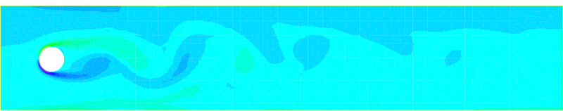
navierStokesEquations — Fig. 166 The vorticity at Reynolds number 100 a time 2s with the Cahouet-Chabart method.

Here you can use the search bar to search in all FreeFEM examples instead

The list of all matching examples on the right is updated for each new query

Clicking on a search hit or on an example on the right brings up the corresponding script from GitHub

You can also filter the list on the right by selecting one or more intersecting categories on the left tree

Navier-Stokes equations

Uzawa Algorithm and Conjugate Gradients

NSUzawaCahouetChabart.edp