Irrotational Fan Blade Flow and Thermal effects

Summary : Here we will learn how to deal with a multi-physics system of PDEs on a complex geometry, with multiple meshes within one problem. We also learn how to manipulate the region indicator and see how smooth is the projection operator from one mesh to another.

Incompressible flow

Without viscosity and vorticity incompressible flows have a velocity given by:

\[\begin{split}\boldsymbol{u}=\left(\begin{matrix}{\partial \psi \over \partial x }\\ -\partial \psi \over \partial y \end{matrix}\right), \quad \mbox{ where }\psi\mbox{ is solution of }\quad \Delta \psi =0\end{split}\]

This equation expresses both incompressibility (\(\nabla\cdot u=0\)) and absence of vortex (\(\nabla\times u =0\)).

As the fluid slips along the walls, normal velocity is zero, which means that \(\psi\) satisfies:

\[\psi \hbox{ constant on the walls}.\]

One can also prescribe the normal velocity at an artificial boundary, and this translates into non constant Dirichlet data for \(\psi\).

Airfoil

Let us consider a wing profile \(S\) in a uniform flow. Infinity will be represented by a large circle \(C\) where the flow is assumed to be of uniform velocity; one way to model this problem is to write:

\[\Delta \psi =0 \hbox{ in } \Omega, \qquad \psi |_{S}=-l, \quad \psi|_{C}= {\boldsymbol{u}_\infty}.\boldsymbol{x}^\perp\]

where \(\partial\Omega=C\cup S\) and \(l\) is the lift force.

The NACA0012 Airfoil

An equation for the upper surface of a NACA0012 (this is a classical wing profile in aerodynamics) is:

\[y = 0.17735\sqrt{x}-0.075597x- 0.212836x^2+0.17363x^3-0.06254x^4.\]

// Parameters
int  S = 99;// wing label
// u infty
real theta = 8*pi/180;// // 1 degree on incidence =>  lift
real lift = theta*0.151952/0.0872665; //  lift approximation formula
real  uinfty1= cos(theta), uinfty2= sin(theta);
// Mesh
func naca12 = 0.17735*sqrt(x) - 0.075597*x - 0.212836*(x^2) + 0.17363*(x^3) - 0.06254*(x^4);
border C(t=0., 2.*pi){x=5.*cos(t); y=5.*sin(t);}
border Splus(t=0., 1.){x=t; y=naca12; label=S;}
border Sminus(t=1., 0.){x=t; y=-naca12; label=S;}
mesh Th = buildmesh(C(50) + Splus(70) + Sminus(70));

// Fespace
fespace Xh(Th, P2);
Xh psi, w;
macro grad(u) [dx(u),dy(u)]// def of grad operator
// Solve
solve potential(psi, w)
   = int2d(Th)(
        grad(psi)'*grad(w) //  scalar product
   )
   + on(C, psi = [uinfty1,uinfty2]'*[y,-x])
   + on(S, psi=-lift) // to get a correct value
   ;

plot(psi, wait=1);

A zoom of the streamlines are shown on Fig. 15.

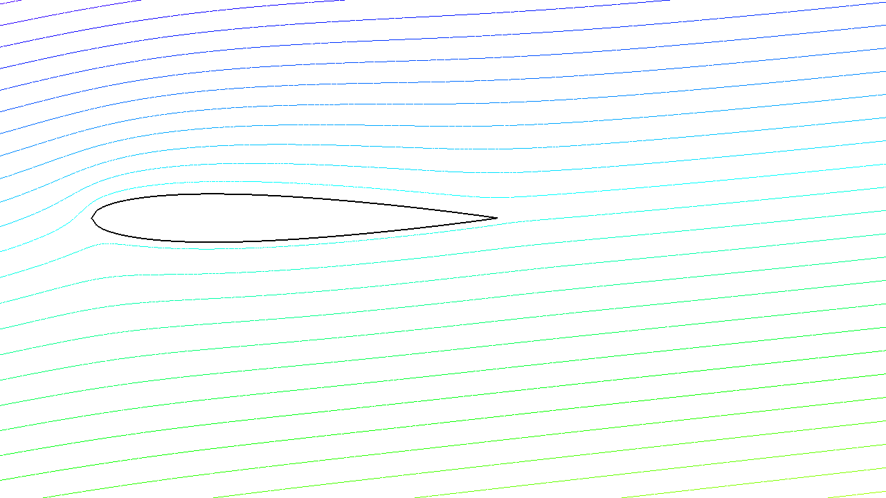
Potential — Fig. 15 Zoom around the NACA0012 airfoil showing the streamlines (curve \(\psi=\) constant). To obtain such a plot use the interactive graphic command: “+” and p.

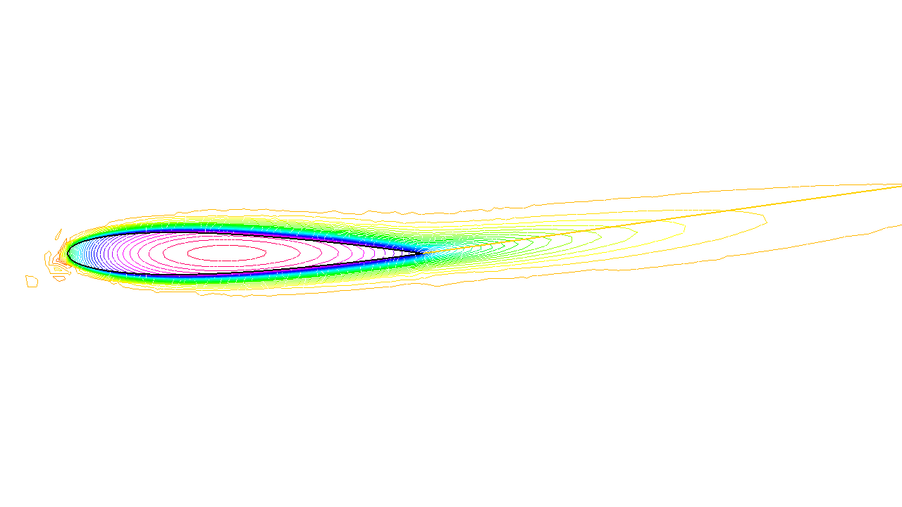
PotentialHeat — Fig. 16 Temperature distribution at time T=25 (now the maximum is at 90 instead of 120).

The NACA0012 Airfoil

Heat Convection around the airfoil

Now let us assume that the airfoil is hot and that air is there to cool it. Much like in the previous section the heat equation for the temperature \(v\) is

\[\partial_t v -\nabla\cdot(\kappa\nabla v) + u\cdot\nabla v =0,~~v(t=0)=v_0, ~~\frac{\partial v}{\partial\boldsymbol{n}}|_{C,u\cdot n>0}=0, v|_{C,u\cdot n<0}=0\]

But now the domain is outside AND inside \(S\) and \(\kappa\) takes a different value in air and in steel. Furthermore there is convection of heat by the flow, hence the term \(u\cdot\nabla v\) above.

Consider the following, to be plugged at the end of the previous program:

// Corrected by F. Hecht may 2021
// Parameters
real S = 99;

border C(t=0, 2*pi){x=3*cos(t); y=3*sin(t);} // Label 1,2
border Splus(t=0, 1){x=t; y=0.17735*sqrt(t) - 0.075597*t - 0.212836*(t^2) + 0.17363*(t^3) - 0.06254*(t^4); label=S;}
border Sminus(t=1, 0){x=t; y=-(0.17735*sqrt(t) - 0.075597*t - 0.212836*(t^2) + 0.17363*(t^3) - 0.06254*(t^4)); label=S;}
mesh Th = buildmesh(C(50) + Splus(70) + Sminus(70));
// Fespace
fespace Vh(Th, P2);
Vh psi, w;

// Problem
solve potential(psi, w)
= int2d(Th)(dx(psi)*dx(w)+dy(psi)*dy(w))
     + on(C, psi = y)
     + on(S, psi=0);

// Plot
plot(psi, wait=1);

/// Thermic
// Parameters
real dt = 0.005, nbT = 50;

// Mesh
border D(t=0, 2){x=1+t; y=0;}
mesh Sh = buildmesh(C(25) + Splus(-90) + Sminus(-90) + D(200));
int steel = Sh(0.5, 0).region, air = Sh(-1, 0).region;
// Change label to put BC on In flow
// Fespace
fespace Wh(Sh, P1);
Wh  vv;

fespace W0(Sh, P0);
W0 k = 0.01*(region == air) + 0.1*(region == steel);
W0 u1 = dy(psi)*(region == air), u2 = -dx(psi)*(region == air);
Wh v = 120*(region == steel), vold;
// set the label to 10 on inflow boundary to inforce the temperature.
Sh = change(Sh,flabel = (label == C &&  [u1,u2]'*N<0) ? 10 : label);
int i;
problem thermic(v, vv, init=i, solver=LU)
= int2d(Sh)(
              v*vv/dt + k*(dx(v)*dx(vv) + dy(v)*dy(vv))
            + 10*(u1*dx(v) + u2*dy(v))*vv
           )
- int2d(Sh)(vold*vv/dt)
+ on(10, v= 0);


for(i = 0; i < nbT; i++) {
  vold[]= v[];
  thermic;
  plot(v);
}

Note

How steel and air are identified by the mesh parameter region which is defined when buildmesh is called and takes an integer value corresponding to each connected component of \(\Omega\);

Note

We use the change function to put label 10 on inflow boundary, remark the trick to chanhe only label C flabel = (label == C && [u1,u2]'*N<0) ? 10 : label

How the convection terms are added without upwinding. Upwinding is necessary when the Pecley number \(|u|L/\kappa\) is large (here is a typical length scale), The factor 10 in front of the convection terms is a quick way of multiplying the velocity by 10 (else it is too slow to see something).

The solver is Gauss’ LU factorization and when init \(\neq 0\) the LU decomposition is reused so it is much faster after the first iteration.

Here you can use the search bar to search in all FreeFEM examples instead

The list of all matching examples on the right is updated for each new query

Clicking on a search hit or on an example on the right brings up the corresponding script from GitHub

You can also filter the list on the right by selecting one or more intersecting categories on the left tree

Irrotational Fan Blade Flow and Thermal effects

Heat Convection around the airfoil