Domain decomposition
We present three classic examples of domain decomposition technique: first, Schwarz algorithm with overlapping, second Schwarz algorithm without overlapping (also call Shur complement), and last we show to use the conjugate gradient to solve the boundary problem of the Shur complement.
Schwarz overlapping
To solve:
the Schwarz algorithm runs like this:
where \(\Gamma_i\) is the boundary of \(\Omega_i\) and on the condition that \(\Omega_1\cap\Omega_2\neq\emptyset\) and that \(u_i\) are zero at iteration 1.
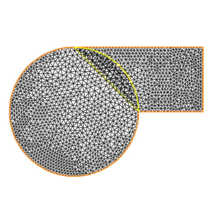
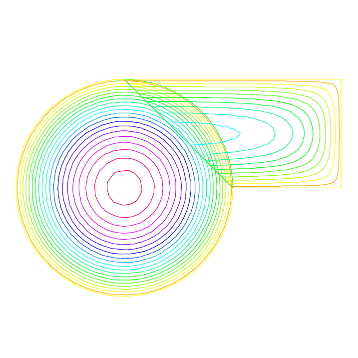
Here we take \(\Omega_1\) to be a quadrangle, \(\Omega_2\) a disk and we apply the algorithm starting from zero.
Tip
Schwarz overlapping
1// Parameters
2int inside =2; //inside boundary
3int outside = 1; //outside boundary
4int n = 4;
5
6// Mesh
7border a(t=1, 2){x=t; y=0; label=outside;}
8border b(t=0, 1){x=2; y=t; label=outside;}
9border c(t=2, 0){x=t; y=1; label=outside;}
10border d(t=1, 0){x=1-t; y=t; label=inside;}
11border e(t=0, pi/2){x=cos(t); y=sin(t); label=inside;}
12border e1(t=pi/2, 2*pi){x=cos(t); y=sin(t); label=outside;}
13mesh th = buildmesh(a(5*n) + b(5*n) + c(10*n) + d(5*n));
14mesh TH = buildmesh(e(5*n) + e1(25*n));
15plot(th, TH, wait=true); //to see the 2 meshes
16
17// Fespace
18fespace vh(th, P1);
19vh u=0, v;
20
21fespace VH(TH, P1);
22VH U, V;
23
24// Problem
25int i = 0;
26problem PB (U, V, init=i, solver=Cholesky)
27 = int2d(TH)(
28 dx(U)*dx(V)
29 + dy(U)*dy(V)
30 )
31 + int2d(TH)(
32 - V
33 )
34 + on(inside, U=u)
35 + on(outside, U=0)
36 ;
37
38problem pb (u, v, init=i, solver=Cholesky)
39 = int2d(th)(
40 dx(u)*dx(v)
41 + dy(u)*dy(v)
42 )
43 + int2d(th)(
44 - v
45 )
46 + on(inside, u=U)
47 + on(outside, u=0)
48 ;
49
50// Calculation loop
51for (i = 0 ; i < 10; i++){
52 // Solve
53 PB;
54 pb;
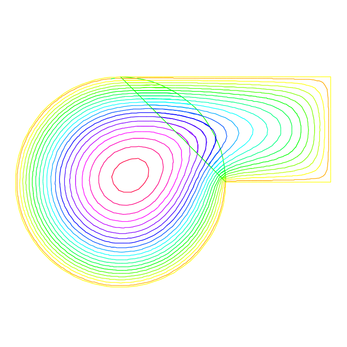
55
56 // Plot
57 plot(U, u, wait=true);
58}
Schwarz non overlapping Scheme
To solve:
the Schwarz algorithm for domain decomposition without overlapping runs like this
Let introduce \(\Gamma_i\) is common the boundary of \(\Omega_1\) and \(\Omega_2\) and \(\Gamma_e^i= \partial \Omega_i \setminus \Gamma_i\).
The problem find \(\lambda\) such that \((u_1|_{\Gamma_i}=u_2|_{\Gamma_i})\) where \(u_i\) is solution of the following Laplace problem:
To solve this problem we just make a loop with upgrading \(\lambda\) with
where the sign \(+\) or \(-\) of \({\pm}\) is choose to have convergence.
Tip
Schwarz non-overlapping
 1// Parameters
 2int inside = 2; int outside = 1; int n = 4;
 3
 4// Mesh
 5border a(t=1, 2){x=t; y=0; label=outside;};
 6border b(t=0, 1){x=2; y=t; label=outside;};
 7border c(t=2, 0){x=t; y=1; label=outside;};
 8border d(t=1, 0){x=1-t; y=t; label=inside;};
 9border e(t=0, 1){x=1-t; y=t; label=inside;};
10border e1(t=pi/2, 2*pi){x=cos(t); y=sin(t); label=outside;};
11mesh th = buildmesh(a(5*n) + b(5*n) + c(10*n) + d(5*n));
12mesh TH = buildmesh(e(5*n) + e1(25*n));
13plot(th, TH, wait=true);
14
15// Fespace
16fespace vh(th, P1);
17vh u=0, v;
18vh lambda=0;
19
20fespace VH(TH, P1);
21VH U, V;
22
23// Problem
24int i = 0;
25problem PB (U, V, init=i, solver=Cholesky)
26    = int2d(TH)(
27          dx(U)*dx(V)
28        + dy(U)*dy(V)
29    )
30    + int2d(TH)(
31        - V
32    )
33    + int1d(TH, inside)(
34          lambda*V
35    )
36    + on(outside, U= 0 )
37    ;
38
39problem pb (u, v, init=i, solver=Cholesky)
40    = int2d(th)(
41          dx(u)*dx(v)
42        + dy(u)*dy(v)
43    )
44    + int2d(th)(
45        - v
46    )
47    + int1d(th, inside)(
48        - lambda*v
49    )
50    + on(outside, u=0)
51    ;
52
53for (i = 0; i < 10; i++){
54    // Solve
55    PB;
56    pb;
57    lambda = lambda - (u-U)/2;
58
59    // Plot
60    plot(U,u,wait=true);
61}
62
63// Plot
64plot(U, u);
Schwarz conjuguate gradient
To solve \(-\Delta u =f \;\mbox{in}\;\Omega=\Omega_1\cup\Omega_2\quad u|_\Gamma=0\) the Schwarz algorithm for domain decomposition without overlapping runs like this
Let introduce \(\Gamma_i\) is common the boundary of \(\Omega_1\) and \(\Omega_2\) and \(\Gamma_e^i= \partial \Omega_i \setminus \Gamma_i\).
The problem find \(\lambda\) such that \((u_1|_{\Gamma_i}=u_2|_{\Gamma_i})\) where \(u_i\) is solution of the following Laplace problem:
The version of this example uses the Shur complement. The problem on the border is solved by a conjugate gradient method.
Tip
Schwarz conjugate gradient
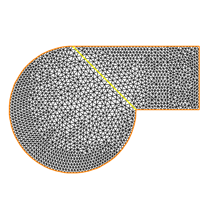
First, we construct the two domains:
 1// Parameters
 2int inside = 2; int outside = 1; int n = 4;
 3
 4// Mesh
 5border Gamma1(t=1, 2){x=t; y=0; label=outside;}
 6border Gamma2(t=0, 1){x=2; y=t; label=outside;}
 7border Gamma3(t=2, 0){x=t; y=1; label=outside;}
 8border GammaInside(t=1, 0){x=1-t; y=t; label=inside;}
 9border GammaArc(t=pi/2, 2*pi){x=cos(t); y=sin(t); label=outside;}
10mesh Th1 = buildmesh(Gamma1(5*n) + Gamma2(5*n) + GammaInside(5*n) + Gamma3(5*n));
11mesh Th2 = buildmesh(GammaInside(-5*n) + GammaArc(25*n));
12plot(Th1, Th2);
Now, define the finite element spaces:
1// Fespace
2fespace Vh1(Th1, P1);
3Vh1 u1, v1;
4Vh1 lambda;
5Vh1 p=0;
6
7fespace Vh2(Th2,P1);
8Vh2 u2, v2;
Note
It is impossible to define a function just on a part of boundary, so the \(\lambda\) function must be defined on the all domain \(\Omega_1\) such as:
1Vh1 lambda;
The two Poisson’s problems:
 1problem Pb1 (u1, v1, init=i, solver=Cholesky)
 2    = int2d(Th1)(
 3          dx(u1)*dx(v1)
 4        + dy(u1)*dy(v1)
 5    )
 6    + int2d(Th1)(
 7        - v1
 8    )
 9    + int1d(Th1, inside)(
10          lambda*v1
11    )
12    + on(outside, u1=0)
13    ;
14
15problem Pb2 (u2, v2, init=i, solver=Cholesky)
16    = int2d(Th2)(
17          dx(u2)*dx(v2)
18        + dy(u2)*dy(v2)
19    )
20    + int2d(Th2)(
21        - v2
22    )
23    + int1d(Th2, inside)(
24        - lambda*v2
25    )
26    + on(outside, u2=0)
27    ;
And, we define a border matrix, because the \(\lambda\) function is none zero inside the domain \(\Omega_1\):
1varf b(u2, v2, solver=CG) = int1d(Th1, inside)(u2*v2);
2matrix B = b(Vh1, Vh1, solver=CG);
The boundary problem function,
 1// Boundary problem function
 2func real[int] BoundaryProblem (real[int] &l){
 3   lambda[] = l; //make FE function form l
 4   Pb1;
 5   Pb2;
 6   i++; //no refactorization i != 0
 7   v1 = -(u1-u2);
 8   lambda[] = B*v1[];
 9   return lambda[];
10}
Note
The difference between the two notations v1 and v1[] is: v1 is the finite element function and v1[] is the vector in the canonical basis of the finite element function v1.
1// Solve
2real cpu=clock();
3LinearCG(BoundaryProblem, p[], eps=1.e-6, nbiter=100);
4//compute the final solution, because CG works with increment
5BoundaryProblem(p[]); //solve again to have right u1, u2
6
7// Display & Plot
8cout << " -- CPU time schwarz-gc:" << clock()-cpu << endl;
9plot(u1, u2);