Mesh Generation
In this section, operators and tools on meshes are presented.
FreeFEM type for mesh variable:
1D mesh:
meshL
2D mesh:
mesh
3D volume mesh:
mesh3- 3D border meshes
3D surface
meshS3D curve
meshL
Through this presentation, the principal commands for the mesh generation and links between mesh - mesh3 - meshS - meshL are described.
The type mesh in 2 dimension
Commands for 2d mesh Generation
The FreeFEM type to define a 2d mesh object is mesh.
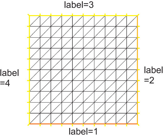
The command square
The command square triangulates the unit square.
The following generates a \(4\times 5\) grid in the unit square \([0,1]^2\). The labels of the boundaries are shown in Fig. 57.
1mesh Th = square(4, 5);
To construct a \(n\times m\) grid in the rectangle \([x_0,x_1]\times [y_0,y_1]\), proceed as follows:
1real x0 = 1.2;
2real x1 = 1.8;
3real y0 = 0;
4real y1 = 1;
5int n = 5;
6real m = 20;
7mesh Th = square(n, m, [x0+(x1-x0)*x, y0+(y1-y0)*y]);
Note
Adding the named parameter flags=icase with icase:
will produce a mesh where all quads are split with diagonal \(x-y=constant\)
will produce a Union Jack flag type of mesh
will produce a mesh where all quads are split with diagonal \(x+y=constant\)
same as in case 0, except two corners where the triangles are the same as case 2, to avoid having 3 vertices on the boundary
same as in case 2, except two corners where the triangles are the same as case 0, to avoid having 3 vertices on the boundary
1mesh Th = square(n, m, [x0+(x1-x0)*x, y0+(y1-y0)*y], flags=icase);
Note
Adding the named parameter label=labs will
change the 4 default label numbers to labs[i-1], for
example int[int] labs=[11, 12, 13, 14], and adding the
named parameter region=10 will change the region number
to \(10\), for instance (v 3.8).
To see all of these flags at work, check Square mesh example:
1for (int i = 0; i < 5; ++i){
2   int[int] labs = [11, 12, 13, 14];
3   mesh Th = square(3, 3, flags=i, label=labs, region=10);
4   plot(Th, wait=1, cmm="square flags = "+i );
5}
The command buildmesh
mesh building with border
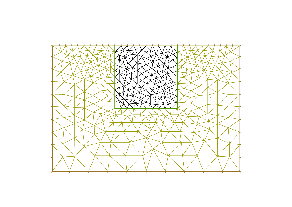
Boundaries are defined piecewise by parametrized curves. The pieces can only intersect at their endpoints, but it is possible to join more than two endpoints. This can be used to structure the mesh if an area touches a border and create new regions by dividing larger ones:
 1int upper = 1;
 2int others = 2;
 3int inner = 3;
 4
 5border C01(t=0, 1){x=0; y=-1+t; label=upper;}
 6border C02(t=0, 1){x=1.5-1.5*t; y=-1; label=upper;}
 7border C03(t=0, 1){x=1.5; y=-t; label=upper;}
 8border C04(t=0, 1){x=1+0.5*t; y=0; label=others;}
 9border C05(t=0, 1){x=0.5+0.5*t; y=0; label=others;}
10border C06(t=0, 1){x=0.5*t; y=0; label=others;}
11border C11(t=0, 1){x=0.5; y=-0.5*t; label=inner;}
12border C12(t=0, 1){x=0.5+0.5*t; y=-0.5; label=inner;}
13border C13(t=0, 1){x=1; y=-0.5+0.5*t; label=inner;}
14
15int n = 10;
16plot(C01(-n) + C02(-n) + C03(-n) + C04(-n) + C05(-n)
17  + C06(-n) + C11(n) + C12(n) + C13(n), wait=true);
18
19mesh Th = buildmesh(C01(-n) + C02(-n) + C03(-n) + C04(-n) + C05(-n)
20  + C06(-n) + C11(n) + C12(n) + C13(n));
21
22plot(Th, wait=true);
23
24cout << "Part 1 has region number " << Th(0.75, -0.25).region << endl;
25cout << "Part 2 has redion number " << Th(0.25, -0.25).region << endl;
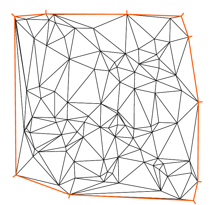
Borders and mesh are respectively shown in Fig. 58 and Fig. 59.
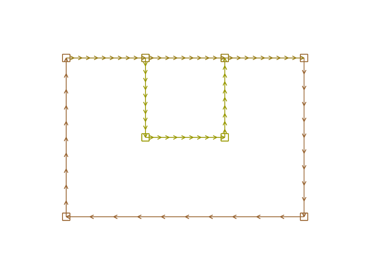
Triangulation keywords assume that the domain is defined as being on the left (resp right) of its oriented parameterized boundary
To check the orientation plot \(t\mapsto (\varphi_x(t),\varphi_y(t)),\, t_0\le t\le t_1\). If it is as in Fig. 60, then the domain lies on the shaded area, otherwise it lies on the opposite side.
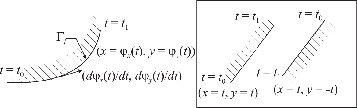
Fig. 60 Orientation of the boundary defined by \((\phi_x(t),\phi_y(t))\)
The general expression to define a triangulation with buildmesh is
1mesh Mesh_Name = buildmesh(Gamma1(m1)+...+GammaJ(mj), OptionalParameter);
where \(m_j\) are positive or negative numbers to indicate how many vertices should be on \(\Gamma_j,\, \Gamma=\cup_{j=1}^J \Gamma_J\), and the optional parameter (see also References), separated with a comma, can be:
nbvx= int, to set the maximum number of vertices in the mesh.fixedborder= bool, to say if the mesh generator can change the boundary mesh or not (by default the boundary mesh can change; beware that with periodic boundary conditions (see. Finite Element), it can be dangerous.
The orientation of boundaries can be changed by changing the sign of \(m_j\).
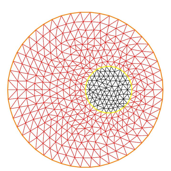
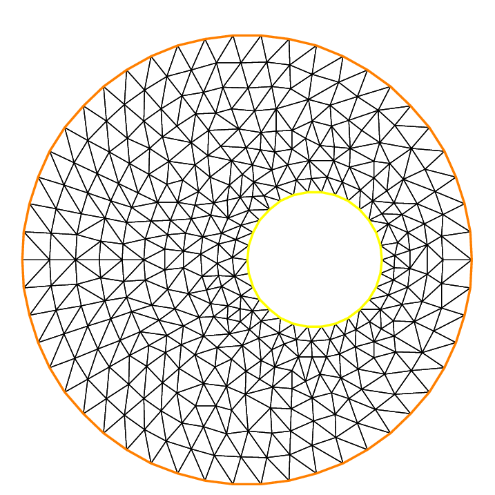
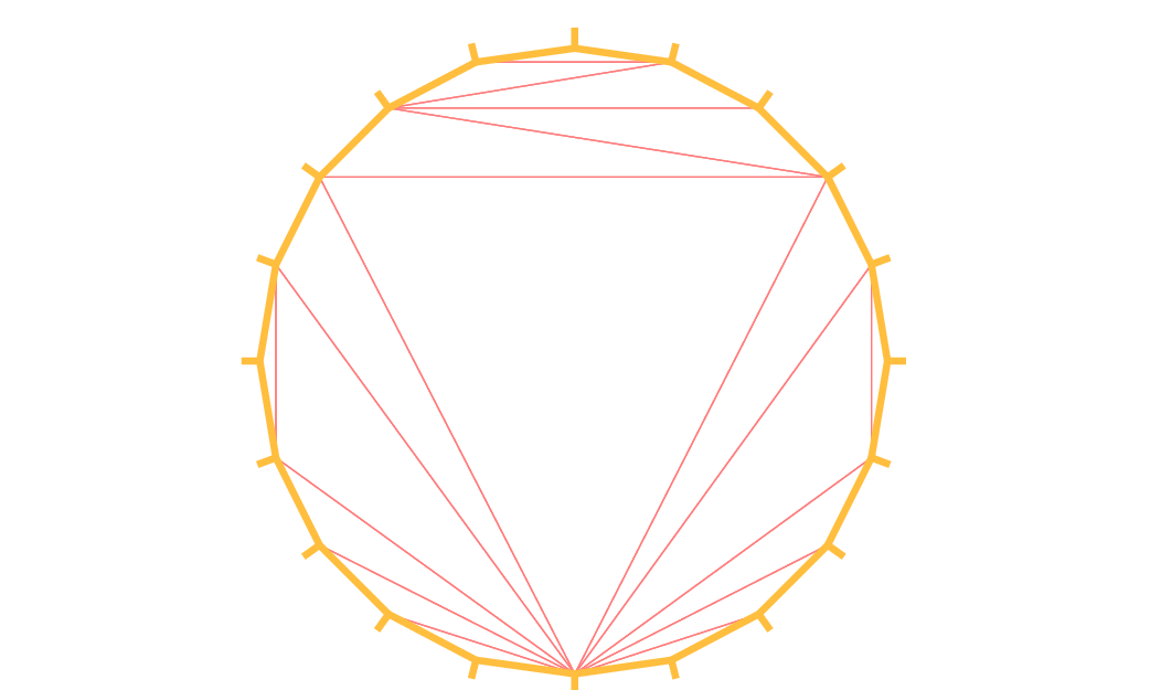
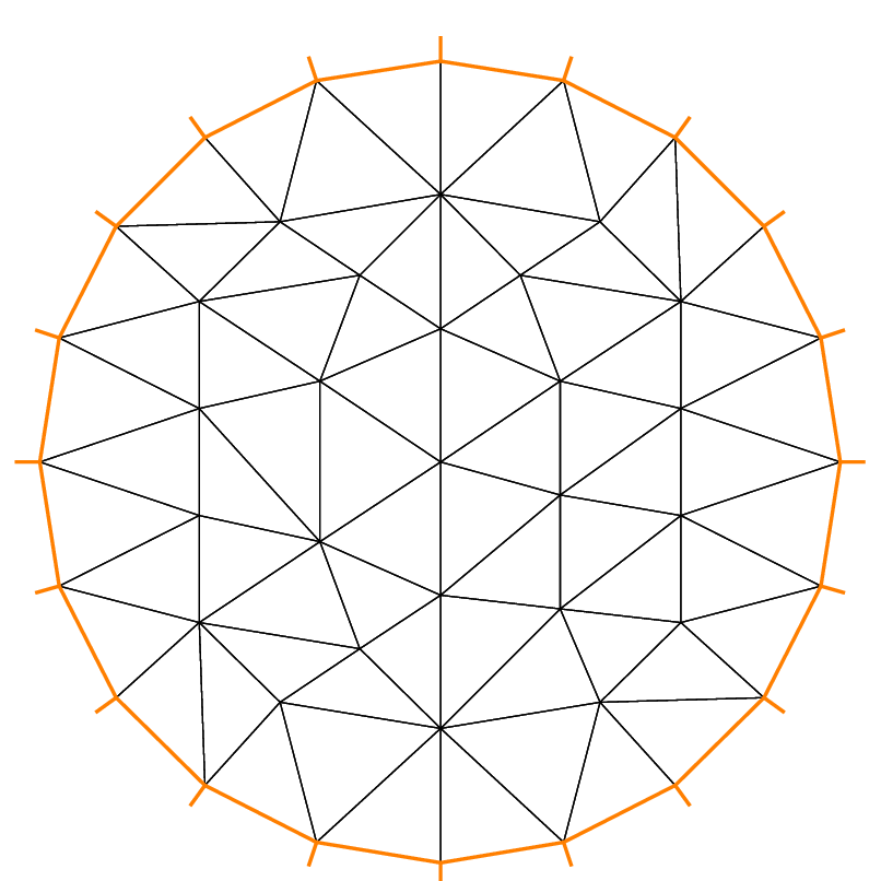
The following example shows how to change the orientation. The example generates the unit disk with a small circular hole, and assigns “1” to the unit disk (“2” to the circle inside). The boundary label must be non-zero, but it can also be omitted.
1border a(t=0, 2*pi){x=cos(t); y=sin(t); label=1;}
2border b(t=0, 2*pi){x=0.3+0.3*cos(t); y=0.3*sin(t); label=2;}
3plot(a(50) + b(30)); //to see a plot of the border mesh
4mesh Thwithouthole = buildmesh(a(50) + b(30));
5mesh Thwithhole = buildmesh(a(50) + b(-30));
6plot(Thwithouthole, ps="Thwithouthole.eps");
7plot(Thwithhole, ps="Thwithhole.eps");
Note
Notice that the orientation is changed by b(-30) in the 5th line. In the 7th line, ps="fileName" is used to generate a postscript file with identification shown on the figure.
Note
Borders are evaluated only at the time plot or buildmesh is called so the global variables are defined at this time. In this case, since \(r\) is changed between the two border calls, the following code will not work because the first border will be computed with r=0.3:
1real r=1;
2border a(t=0, 2*pi){x=r*cos(t); y=r*sin(t); label=1;}
3r=0.3;
4border b(t=0, 2*pi){x=r*cos(t); y=r*sin(t); label=1;}
5mesh Thwithhole = buildmesh(a(50) + b(-30)); // bug (a trap) because
6    // the two circles have the same radius = :math:`0.3`
mesh building with array of border
Sometimes it can be useful to make an array of the border, but unfortunately it is incompatible with the FreeFEM syntax. To bypass this problem, if the number of segments of the discretization \(n\) is an array, we make an implicit loop on all of the values of the array, and the index variable \(i\) of the loop is defined after the parameter definition, like in border a(t=0, 2*pi; i) …
A first very small example:
1border a(t=0, 2*pi; i){x=(i+1)*cos(t); y=(i+1)*sin(t); label=1;}
2int[int] nn = [10, 20, 30];
3plot(a(nn)); //plot 3 circles with 10, 20, 30 points
And a more complex example to define a square with small circles:
 1real[int] xx = [0, 1, 1, 0],
 2          yy = [0, 0, 1, 1];
 3//radius, center of the 4 circles
 4real[int] RC = [0.1, 0.05, 0.05, 0.1],
 5          XC = [0.2, 0.8, 0.2, 0.8],
 6          YC = [0.2, 0.8, 0.8, 0.2];
 7int[int] NC = [-10,-11,-12,13]; //list number of :math:`\pm` segments of the 4 circles borders
 8
 9border bb(t=0, 1; i)
10{
11    // i is the index variable of the multi border loop
12    int ii = (i+1)%4;
13    real t1 = 1-t;
14    x = xx[i]*t1 + xx[ii]*t;
15    y = yy[i]*t1 + yy[ii]*t;
16    label = 0;
17}
18
19border cc(t=0, 2*pi; i)
20{
21    x = RC[i]*cos(t) + XC[i];
22    y = RC[i]*sin(t) + YC[i];
23    label = i + 1;
24}
25int[int] nn = [4, 4, 5, 7]; //4 border, with 4, 4, 5, 7 segment respectively
26plot(bb(nn), cc(NC), wait=1);
27mesh th = buildmesh(bb(nn) + cc(NC));
28plot(th, wait=1);
Mesh Connectivity and data
The following example explains methods to obtain mesh information.
  1// Mesh
  2mesh Th = square(2, 2);
  3
  4cout << "// Get data of the mesh" << endl;
  5{
  6    int NbTriangles = Th.nt;
  7    real MeshArea = Th.measure;
  8    real BorderLength = Th.bordermeasure;
  9
 10    cout << "Number of triangle(s) = " << NbTriangles << endl;
 11    cout << "Mesh area = " << MeshArea << endl;
 12    cout << "Border length = " << BorderLength << endl;
 13
 14    // Th(i) return the vextex i of Th
 15    // Th[k] return the triangle k of Th
 16    // Th[k][i] return the vertex i of the triangle k of Th
 17    for (int i = 0; i < NbTriangles; i++)
 18        for (int j = 0; j < 3; j++)
 19            cout << i << " " << j << " - Th[i][j] = " << Th[i][j]
 20                 << ", x = " << Th[i][j].x
 21                 << ", y= " << Th[i][j].y
 22                 << ", label=" << Th[i][j].label << endl;
 23}
 24
 25cout << "// Hack to get vertex coordinates" << endl;
 26{
 27    fespace femp1(Th, P1);
 28    femp1 Thx=x,Thy=y;
 29
 30    int NbVertices = Th.nv;
 31    cout << "Number of vertices = " << NbVertices << endl;
 32
 33    for (int i = 0; i < NbVertices; i++)
 34        cout << "Th(" << i << ") : " << Th(i).x << " " << Th(i).y << " " << Th(i).label
 35             << endl << "\told method: " << Thx[][i] << " " << Thy[][i] << endl;
 36}
 37
 38cout << "// Method to find information of point (0.55,0.6)" << endl;
 39{
 40    int TNumber = Th(0.55, 0.6).nuTriangle; //the triangle number
 41    int RLabel = Th(0.55, 0.6).region; //the region label
 42
 43    cout << "Triangle number in point (0.55, 0.6): " << TNumber << endl;
 44    cout << "Region label in point (0.55, 0.6): " << RLabel << endl;
 45}
 46
 47cout << "// Information of triangle" << endl;
 48{
 49    int TNumber = Th(0.55, 0.6).nuTriangle;
 50    real TArea = Th[TNumber].area; //triangle area
 51    real TRegion = Th[TNumber].region; //triangle region
 52    real TLabel = Th[TNumber].label; //triangle label, same as region for triangles
 53
 54    cout << "Area of triangle " << TNumber << ": " << TArea << endl;
 55    cout << "Region of triangle " << TNumber << ": " << TRegion << endl;
 56    cout << "Label of triangle " << TNumber << ": " << TLabel << endl;
 57}
 58
 59cout << "// Hack to get a triangle containing point x, y or region number (old method)" << endl;
 60{
 61    fespace femp0(Th, P0);
 62    femp0 TNumbers; //a P0 function to get triangle numbering
 63    for (int i = 0; i < Th.nt; i++)
 64        TNumbers[][i] = i;
 65    femp0 RNumbers = region; //a P0 function to get the region number
 66
 67    int TNumber = TNumbers(0.55, 0.6); // Number of the triangle containing (0.55, 0,6)
 68    int RNumber = RNumbers(0.55, 0.6); // Number of the region containing (0.55, 0,6)
 69
 70    cout << "Point (0.55,0,6) :" << endl;
 71    cout << "\tTriangle number = " << TNumber << endl;
 72    cout << "\tRegion number = " << RNumber << endl;
 73}
 74
 75cout << "// New method to get boundary information and mesh adjacent" << endl;
 76{
 77    int k = 0;
 78    int l=1;
 79    int e=1;
 80
 81    // Number of boundary elements
 82    int NbBoundaryElements = Th.nbe;
 83    cout << "Number of boundary element = " << NbBoundaryElements << endl;
 84    // Boundary element k in {0, ..., Th.nbe}
 85    int BoundaryElement = Th.be(k);
 86    cout << "Boundary element " << k << " = " << BoundaryElement << endl;
 87    // Vertice l in {0, 1} of boundary element k
 88    int Vertex = Th.be(k)[l];
 89    cout << "Vertex " << l << " of boundary element " << k << " = " << Vertex << endl;
 90    // Triangle containg the boundary element k
 91    int Triangle = Th.be(k).Element;
 92    cout << "Triangle containing the boundary element " << k << " = " << Triangle << endl;
 93    // Triangle egde nubmer containing the boundary element k
 94    int Edge = Th.be(k).whoinElement;
 95    cout << "Triangle edge number containing the boundary element " << k << " = " << Edge << endl;
 96    // Adjacent triangle of the triangle k by edge e
 97    int Adjacent = Th[k].adj(e); //The value of e is changed to the corresponding edge in the adjacent triangle
 98    cout << "Adjacent triangle of the triangle " << k << " by edge " << e << " = " << Adjacent << endl;
 99    cout << "\tCorresponding edge = " << e << endl;
100    // If there is no adjacent triangle by edge e, the same triangle is returned
101    //Th[k] == Th[k].adj(e)
102    // Else a different triangle is returned
103    //Th[k] != Th[k].adj(e)
104}
105
106cout << "// Print mesh connectivity " << endl;
107{
108    int NbTriangles = Th.nt;
109    for (int k = 0; k < NbTriangles; k++)
110        cout << k << " : " << int(Th[k][0]) << " " << int(Th[k][1])
111             << " " << int(Th[k][2])
112             << ", label " << Th[k].label << endl;
113
114    for (int k = 0; k < NbTriangles; k++)
115        for (int e = 0, ee; e < 3; e++)
116            //set ee to e, and ee is change by method adj,
117            cout << k << " " << e << " <=> " << int(Th[k].adj((ee=e))) << " " << ee
118                 << ", adj: " << (Th[k].adj((ee=e)) != Th[k]) << endl;
119
120    int NbBoundaryElements = Th.nbe;
121    for (int k = 0; k < NbBoundaryElements; k++)
122        cout << k << " : " << Th.be(k)[0] << " " << Th.be(k)[1]
123             << " , label " << Th.be(k).label
124             << ", triangle " << int(Th.be(k).Element)
125             << " " << Th.be(k).whoinElement << endl;
126
127    real[int] bb(4);
128    boundingbox(Th, bb);
129    // bb[0] = xmin, bb[1] = xmax, bb[2] = ymin, bb[3] =ymax
130    cout << "boundingbox:" << endl;
131    cout << "xmin = " << bb[0]
132         << ", xmax = " << bb[1]
133         << ", ymin = " << bb[2]
134         << ", ymax = " << bb[3] << endl;
135}
The output is:
  1// Get data of the mesh
  2Number of triangle = 8
  3Mesh area = 1
  4Border length = 4
  50 0 - Th[i][j] = 0, x = 0, y= 0, label=4
  60 1 - Th[i][j] = 1, x = 0.5, y= 0, label=1
  70 2 - Th[i][j] = 4, x = 0.5, y= 0.5, label=0
  81 0 - Th[i][j] = 0, x = 0, y= 0, label=4
  91 1 - Th[i][j] = 4, x = 0.5, y= 0.5, label=0
 101 2 - Th[i][j] = 3, x = 0, y= 0.5, label=4
 112 0 - Th[i][j] = 1, x = 0.5, y= 0, label=1
 122 1 - Th[i][j] = 2, x = 1, y= 0, label=2
 132 2 - Th[i][j] = 5, x = 1, y= 0.5, label=2
 143 0 - Th[i][j] = 1, x = 0.5, y= 0, label=1
 153 1 - Th[i][j] = 5, x = 1, y= 0.5, label=2
 163 2 - Th[i][j] = 4, x = 0.5, y= 0.5, label=0
 174 0 - Th[i][j] = 3, x = 0, y= 0.5, label=4
 184 1 - Th[i][j] = 4, x = 0.5, y= 0.5, label=0
 194 2 - Th[i][j] = 7, x = 0.5, y= 1, label=3
 205 0 - Th[i][j] = 3, x = 0, y= 0.5, label=4
 215 1 - Th[i][j] = 7, x = 0.5, y= 1, label=3
 225 2 - Th[i][j] = 6, x = 0, y= 1, label=4
 236 0 - Th[i][j] = 4, x = 0.5, y= 0.5, label=0
 246 1 - Th[i][j] = 5, x = 1, y= 0.5, label=2
 256 2 - Th[i][j] = 8, x = 1, y= 1, label=3
 267 0 - Th[i][j] = 4, x = 0.5, y= 0.5, label=0
 277 1 - Th[i][j] = 8, x = 1, y= 1, label=3
 287 2 - Th[i][j] = 7, x = 0.5, y= 1, label=3
 29// Hack to get vertex coordinates
 30Number of vertices = 9
 31Th(0) : 0 0 4
 32   old method: 0 0
 33Th(1) : 0.5 0 1
 34   old method: 0.5 0
 35Th(2) : 1 0 2
 36   old method: 1 0
 37Th(3) : 0 0.5 4
 38   old method: 0 0.5
 39Th(4) : 0.5 0.5 0
 40   old method: 0.5 0.5
 41Th(5) : 1 0.5 2
 42   old method: 1 0.5
 43Th(6) : 0 1 4
 44   old method: 0 1
 45Th(7) : 0.5 1 3
 46   old method: 0.5 1
 47Th(8) : 1 1 3
 48   old method: 1 1
 49// Method to find the information of point (0.55,0.6)
 50Triangle number in point (0.55, 0.6): 7
 51Region label in point (0.55, 0.6): 0
 52// Information of a triangle
 53Area of triangle 7: 0.125
 54Region of triangle 7: 0
 55Label of triangle 7: 0
 56// Hack to get a triangle containing point x, y or region number (old method)
 57Point (0.55,0,6) :
 58   Triangle number = 7
 59   Region number = 0
 60// New method to get boundary information and mesh adjacent
 61Number of boundary element = 8
 62Boundary element 0 = 0
 63Vertex 1 of boundary element 0 = 1
 64Triangle containing the boundary element 0 = 0
 65Triangle edge number containing the boundary element 0 = 2
 66Adjacent triangle of the triangle 0 by edge 1 = 1
 67   Corresponding edge = 2
 68// Print mesh connectivity
 690 : 0 1 4, label 0
 701 : 0 4 3, label 0
 712 : 1 2 5, label 0
 723 : 1 5 4, label 0
 734 : 3 4 7, label 0
 745 : 3 7 6, label 0
 756 : 4 5 8, label 0
 767 : 4 8 7, label 0
 770 0 <=> 3 1, adj: 1
 780 1 <=> 1 2, adj: 1
 790 2 <=> 0 2, adj: 0
 801 0 <=> 4 2, adj: 1
 811 1 <=> 1 1, adj: 0
 821 2 <=> 0 1, adj: 1
 832 0 <=> 2 0, adj: 0
 842 1 <=> 3 2, adj: 1
 852 2 <=> 2 2, adj: 0
 863 0 <=> 6 2, adj: 1
 873 1 <=> 0 0, adj: 1
 883 2 <=> 2 1, adj: 1
 894 0 <=> 7 1, adj: 1
 904 1 <=> 5 2, adj: 1
 914 2 <=> 1 0, adj: 1
 925 0 <=> 5 0, adj: 0
 935 1 <=> 5 1, adj: 0
 945 2 <=> 4 1, adj: 1
 956 0 <=> 6 0, adj: 0
 966 1 <=> 7 2, adj: 1
 976 2 <=> 3 0, adj: 1
 987 0 <=> 7 0, adj: 0
 997 1 <=> 4 0, adj: 1
1007 2 <=> 6 1, adj: 1
1010 : 0 1 , label 1, triangle 0 2
1021 : 1 2 , label 1, triangle 2 2
1032 : 2 5 , label 2, triangle 2 0
1043 : 5 8 , label 2, triangle 6 0
1054 : 6 7 , label 3, triangle 5 0
1065 : 7 8 , label 3, triangle 7 0
1076 : 0 3 , label 4, triangle 1 1
1087 : 3 6 , label 4, triangle 5 1
109boundingbox:
110xmin = 0, xmax = 1, ymin = 0, ymax = 1
The real characteristic function of a mesh Th is chi(Th) in 2D and 3D where:
chi(Th)(P)=1 if \(P\in Th\)
chi(Th)(P)=0 if \(P\not\in Th\)
The keyword “triangulate”
FreeFEM is able to build a triangulation from a set of points. This triangulation is a Delaunay mesh of the convex hull of the set of points. It can be useful to build a mesh from a table function.
The coordinates of the points and the value of the table function are defined separately with rows of the form: x y f(x,y) in a file such as:
10.51387 0.175741 0.636237
20.308652 0.534534 0.746765
30.947628 0.171736 0.899823
40.702231 0.226431 0.800819
50.494773 0.12472 0.580623
60.0838988 0.389647 0.456045
7...............
The third column of each line is left untouched by the triangulate command.
But you can use this third value to define a table function with rows of the form: x y f(x,y).
The following example shows how to make a mesh from the file xyf with the format stated just above.
The command triangulate only uses the 1st and 2nd columns.
 1// Build the Delaunay mesh of the convex hull
 2mesh Thxy=triangulate("xyf"); //points are defined by the first 2 columns of file `xyf`
 3
 4// Plot the created mesh
 5plot(Thxy);
 6
 7// Fespace
 8fespace Vhxy(Thxy, P1);
 9Vhxy fxy;
10
11// Reading the 3rd column to define the function fxy
12{
13    ifstream file("xyf");
14    real xx, yy;
15    for(int i = 0; i < fxy.n; i++)
16        file >> xx >> yy >> fxy[][i]; //to read third row only.
17                                      //xx and yy are just skipped
18}
19
20// Plot
21plot(fxy);
One new way to build a mesh is to have two arrays: one for the \(x\) values and the other for the \(y\) values.
1//set two arrays for the x's and y's
2Vhxy xx=x, yy=y;
3//build the mesh
4mesh Th = triangulate(xx[], yy[]);
2d Finite Element space on a boundary
To define a Finite Element space on a boundary, we came up with the idea of a mesh with no internal points (called empty mesh). It can be useful to handle Lagrange multipliers in mixed and mortar methods.
So the function emptymesh removes all the internal points of a mesh except points on internal boundaries.
1{
2    border a(t=0, 2*pi){x=cos(t); y=sin(t); label=1;}
3    mesh Th = buildmesh(a(20));
4    Th = emptymesh(Th);
5    plot(Th);
6}
It is also possible to build an empty mesh of a pseudo subregion with emptymesh(Th, ssd) using the set of edges from the mesh Th; an edge \(e\) is in this set when, with the two adjacent triangles \(e =t1\cap t2\) and \(ssd[T1] \neq ssd[T2]\) where \(ssd\) refers to the pseudo region numbering of triangles, they are stored in the int[int] array of size “the number of triangles”.
 1{
 2    mesh Th = square(10, 10);
 3    int[int] ssd(Th.nt);
 4    //build the pseudo region numbering
 5    for(int i = 0; i < ssd.n; i++){
 6        int iq = i/2; //because 2 triangles per quad
 7        int ix = iq%10;
 8        int iy = iq/10;
 9        ssd[i] = 1 + (ix>=5) + (iy>=5)*2;
10    }
11    //build emtpy with all edges $e=T1 \cap T2$ and $ssd[T1] \neq ssd[T2]$
12    Th = emptymesh(Th, ssd);
13    //plot
14    plot(Th);
15    savemesh(Th, "emptymesh.msh");
16}
Remeshing
The command movemesh
Meshes can be translated, rotated, and deformed by movemesh; this is useful for elasticity to watch the deformation due to the displacement \(\mathbf{\Phi}(x,y)=(\Phi_1(x,y),\Phi_2(x,y))\) of shape.
It is also useful to handle free boundary problems or optimal shape problems.
If \(\Omega\) is triangulated as \(T_h(\Omega)\), and \(\mathbf{\Phi}\) is a displacement vector then \(\mathbf{\Phi}(T_h)\) is obtained by:
1mesh Th = movemesh(Th,[Phi1, Phi2]);
Sometimes the transformed mesh is invalid because some triangles have flipped over (meaning it now has a negative area).
To spot such problems, one may check the minimum triangle area in the transformed mesh with checkmovemesh before any real transformation.
For example:
for a big number \(k>1\).
1verbosity = 4;
2
3// Parameters
4real coef = 1;
5
6// Mesh
7border a(t=0, 1){x=t; y=0; label=1;};
8border b(t=0, 0.5){x=1; y=t; label=1;};
9border c(t=0, 0.5){x=1-t; y=0.5; label=1;};
10border d(t=0.5, 1){x=0.5; y=t; label=1;};
11border e(t=0.5, 1){x=1-t; y=1; label=1;};
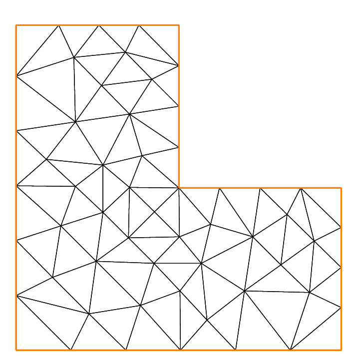
12border f(t=0, 1){x=0; y=1-t; label=1;};
13mesh Th = buildmesh(a(6) + b(4) + c(4) + d(4) + e(4) + f(6));
14plot(Th, wait=true, fill=true, ps="Lshape.eps");
15
16// Function
17func uu = sin(y*pi)/10;
18func vv = cos(x*pi)/10;
19
20// Checkmovemesh
21real minT0 = checkmovemesh(Th, [x, y]); //return the min triangle area
22while(1){ // find a correct move mesh
23 real minT = checkmovemesh(Th, [x+coef*uu, y+coef*vv]);
24 if (minT > minT0/5) break; //if big enough
25 coef /= 1.5;
26}
27
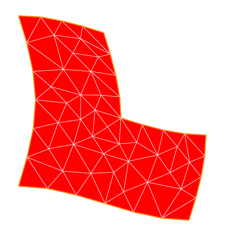
28// Movemesh
29Th = movemesh(Th, [x+coef*uu, y+coef*vv]);
30plot(Th, wait=true, fill=true, ps="MovedMesh.eps");
Note
Consider a function \(u\) defined on a mesh Th.
A statement like Th=movemesh(Th...) does not change \(u\) and so the old mesh still exists.
It will be destroyed when no function uses it.
A statement like \(u=u\) redefines \(u\) on the new mesh Th with interpolation and therefore destroys the old Th, if \(u\) was the only function using it.
Now, we give an example of moving a mesh with a Lagrangian function \(u\) defined on the moving mesh.
 1// Parameters
 2int nn = 10;
 3real dt = 0.1;
 4
 5// Mesh
 6mesh Th = square(nn, nn);
 7
 8// Fespace
 9fespace Vh(Th, P1);
10Vh u=y;
11
12// Loop
13real t=0;
14for (int i = 0; i < 4; i++){
15    t = i*dt;
16    Vh f=x*t;
17    real minarea = checkmovemesh(Th, [x, y+f]);
18    if (minarea > 0) //movemesh will be ok
19    Th = movemesh(Th, [x, y+f]);
20
21    cout << " Min area = " << minarea << endl;
22
23    real[int] tmp(u[].n);
24    tmp = u[]; //save the value
25    u = 0;//to change the FEspace and mesh associated with u
26    u[] = tmp;//set the value of u without any mesh update
27    plot(Th, u, wait=true);
28}
29// In this program, since u is only defined on the last mesh, all the
30// previous meshes are deleted from memory.
The command hTriangle
This section presents the way to obtain a regular triangulation with FreeFEM.
For a set \(S\), we define the diameter of \(S\) by
The sequence \(\{\mathcal{T}_h\}_{h\rightarrow 0}\) of \(\Omega\) is called regular if they satisfy the following:
\(\lim_{h\rightarrow 0}\max\{\textrm{diam}(T_k)|\; T_k\in \mathcal{T}_h\}=0\)
There is a number \(\sigma>0\) independent of \(h\) such that \(\frac{\rho(T_k)}{\textrm{diam}(T_k)}\ge \sigma\quad \textrm{for all }T_k\in \mathcal{T}_h\) where \(\rho(T_k)\) are the diameter of the inscribed circle of \(T_k\).
We put \(h(\mathcal{T}_h)=\max\{\textrm{diam}(T_k)|\; T_k\in \mathcal{T}_h\}\), which is obtained by
1mesh Th = ......;
2fespace Ph(Th, P0);
3Ph h = hTriangle;
4cout << "size of mesh = " << h[].max << endl;
The command adaptmesh
The function:
sharply varies in value and the initial mesh given by one of the commands in the Mesh Generation part cannot reflect its sharp variations.
 1// Parameters
 2real eps = 0.0001;
 3real h = 1;
 4real hmin = 0.05;
 5func f = 10.0*x^3 + y^3 + h*atan2(eps, sin(5.0*y)-2.0*x);
 6
 7// Mesh
 8mesh Th = square(5, 5, [-1+2*x, -1+2*y]);
 9
10// Fespace
11fespace Vh(Th,P1);
12Vh fh = f;
13plot(fh);
14
15// Adaptmesh
16for (int i = 0; i < 2; i++){
17    Th = adaptmesh(Th, fh);
18    fh = f; //old mesh is deleted
19    plot(Th, fh, wait=true);
20}
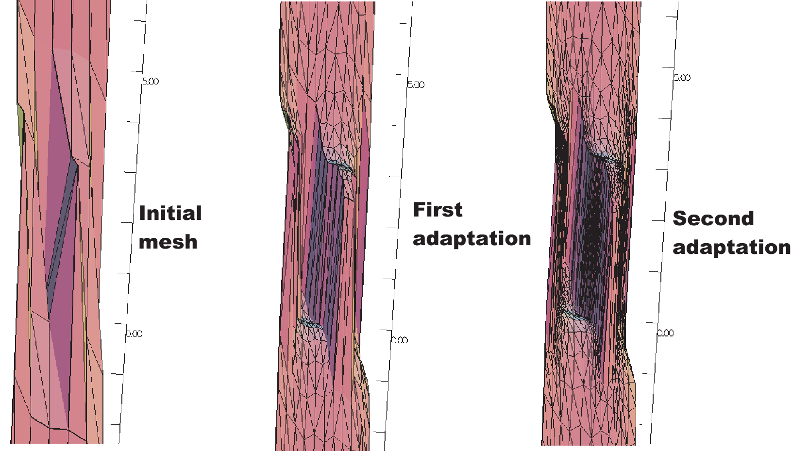
Fig. 69 3D graphs for the initial mesh and 1st and 2nd mesh adaptations
FreeFEM uses a variable metric/Delaunay automatic meshing algorithm.
The command:
1mesh ATh = adaptmesh(Th, f);
create the new mesh ATh adapted to the Hessian
of a function (formula or FE-function).
Mesh adaptation is a very powerful tool when the solution of a problem varies locally and sharply.
Here we solve the Poisson’s problem, when \(f=1\) and \(\Omega\) is an L-shape domain.
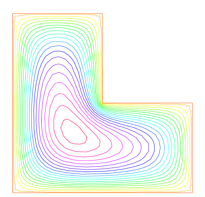
Mesh adaptation
Tip
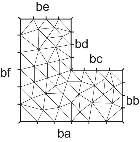
The solution has the singularity \(r^{3/2},\, r=|x-\gamma|\) at the point \(\gamma\) of the intersection of two lines \(bc\) and \(bd\) (see Fig. 70).
 1// Parameters
 2real error = 0.1;
 3
 4// Mesh
 5border ba(t=0, 1){x=t; y=0; label=1;}
 6border bb(t=0, 0.5){x=1; y=t; label=1;}
 7border bc(t=0, 0.5){x=1-t; y=0.5; label=1;}
 8border bd(t=0.5, 1){x=0.5; y=t; label=1;}
 9border be(t=0.5, 1){x=1-t; y=1; label=1;}
10border bf(t=0, 1){x=0; y=1-t; label=1;}
11mesh Th = buildmesh(ba(6) + bb(4) + bc(4) + bd(4) + be(4) + bf(6));
12
13// Fespace
14fespace Vh(Th, P1);
15Vh u, v;
16
17// Function
18func f = 1;
19
20// Problem
21problem Poisson(u, v, solver=CG, eps=1.e-6)
22    = int2d(Th)(
23          dx(u)*dx(v)
24        + dy(u)*dy(v)
25    )
26    - int2d(Th)(
27          f*v
28    )
29    + on(1, u=0);
30
31// Adaptmesh loop
32for (int i = 0; i < 4; i++){
33    Poisson;
34    Th = adaptmesh(Th, u, err=error);
35    error = error/2;
36}
37
38// Plot
39plot(u);
To speed up the adaptation, the default parameter err of adaptmesh is changed by hand; it specifies the required precision, so as to make the new mesh finer or coarser.
The problem is coercive and symmetric, so the linear system can be solved with the conjugate gradient method (parameter solver=CG) with the stopping criteria on the residual, here eps=1.e-6).
By adaptmesh, the slope of the final solution is correctly computed near the point of intersection of \(bc\) and \(bd\) as in Fig. 71.
This method is described in detail in [HECHT1998]. It has a number of default parameters which can be modified.
If f1,f2 are functions and thold, Thnew are meshes:
1   Thnew = adaptmesh(Thold, f1 ... );
2   Thnew = adaptmesh(Thold, f1,f2 ... ]);
3   Thnew = adaptmesh(Thold, [f1,f2] ... );
The additional parameters of adaptmesh are:
See Reference part for more inforamtions
hmin=Minimum edge size.Its default is related to the size of the domain to be meshed and the precision of the mesh generator.
hmax=Maximum edge size.It defaults to the diameter of the domain to be meshed.
err=\(P_1\) interpolation error level (0.01 is the default).errg=Relative geometrical error.By default this error is 0.01, and in any case it must be lower than \(1/\sqrt{2}\). Meshes created with this option may have some edges smaller than the
-hmindue to geometrical constraints.
nbvx=Maximum number of vertices generated by the mesh generator (9000 is the default).nbsmooth=number of iterations of the smoothing procedure (5 is the default).nbjacoby=number of iterations in a smoothing procedure during the metric construction, 0 means no smoothing, 6 is the default.ratio=ratio for a prescribed smoothing on the metric.If the value is 0 or less than 1.1 no smoothing is done on the metric. 1.8 is the default. If
ratio > 1.1, the speed of mesh size variations is bounded by \(log(\mathtt{ratio})\).Note
As
ratiogets closer to 1, the number of generated vertices increases. This may be useful to control the thickness of refined regions near shocks or boundary layers.
omega=relaxation parameter for the smoothing procedure. 1.0 is the default.iso=If true, forces the metric to be isotropic.falseis the default.abserror=If false, the metric is evaluated using the criteria of equi-repartion of relative error.falseis the default. In this case the metric is defined by:\[\mathcal{M} = \left({1\over\mathtt{err}\,\, \mathtt{coef}^2} \quad { |\mathcal{H}| \over max(\mathtt{CutOff},|\eta|)}\right)^p\]Otherwise, the metric is evaluated using the criteria of equi-distribution of errors. In this case the metric is defined by:
\[\mathcal{M} = \left({1\over \mathtt{err}\,\,\mathtt{coef}^2} \quad {|{\mathcal{H}|} \over {\sup(\eta)-\inf(\eta)}}\right)^p.\label{eq err abs}\]
cutoff=lower limit for the relative error evaluation. 1.0e-6 is the default.verbosity=informational messages level (can be chosen between 0 and \(\infty\)).Also changes the value of the global variable verbosity (obsolete).
inquire=To inquire graphically about the mesh.falseis the default.splitpbedge=If true, splits all internal edges in half with two boundary vertices.trueis the default.
maxsubdiv=Changes the metric such that the maximum subdivision of a background edge is bound byval.Always limited by 10, and 10 is also the default.
rescaling=if true, the function, with respect to which the mesh is adapted, is rescaled to be between 0 and 1.trueis the default.
keepbackvertices=if true, tries to keep as many vertices from the original mesh as possible.trueis the default.
IsMetric=if true, the metric is defined explicitly.falseis the default. If the 3 functions \(m_{11}, m_{12}, m_{22}\) are given, they directly define a symmetric matrix field whose Hessian is computed to define a metric. If only one function is given, then it represents the isotropic mesh size at every point.For example, if the partial derivatives
fxx(\(=\partial^2 f/\partial x^2\)),fxy(\(=\partial^2 f/\partial x\partial y\)),fyy(\(=\partial^2 f/\partial y^2\)) are given, we can setTh = adaptmesh(Th, fxx, fxy, fyy, IsMetric=1, nbvx=10000, hmin=hmin);
power=exponent power of the Hessian used to compute the metric.1 is the default.
thetamax=minimum corner angle in degrees.Default is \(10^\circ\) where the corner is \(ABC\) and the angle is the angle of the two vectors \({AB}, {BC}\), (\(0\) imply no corner, \(90\) imply perpendicular corner, …).
splitin2=boolean value.If true, splits all triangles of the final mesh into 4 sub-triangles.
metric=an array of 3 real arrays to set or get metric data information.The size of these three arrays must be the number of vertices. So if
m11,m12,m22are three P1 finite elements related to the mesh to adapt, you can write:metric=[m11[],m12[],m22[]](see fileconvect-apt.edpfor a full example)
nomeshgeneration=If true, no adapted mesh is generated (useful to compute only a metric).periodic=Writingperiodic=[[4,y],[2,y],[1,x],[3,x]];builds an adapted periodic mesh.The sample builds a biperiodic mesh of a square. (see periodic finite element spaces, and see the Sphere example for a full example)
We can use the command adaptmesh to build a uniform mesh with a constant mesh size.
To build a mesh with a constant mesh size equal to \(\frac{1}{30}\) try:
1mesh Th=square(2, 2); //the initial mesh
2plot(Th, wait=true, ps="square-0.eps");
3
4Th = adaptmesh(Th, 1./30., IsMetric=1, nbvx=10000);
5plot(Th, wait=true, ps="square-1.eps");
6
7Th = adaptmesh(Th, 1./30., IsMetric=1, nbvx=10000); //More the one time du to
8Th = adaptmesh(Th, 1./30., IsMetric=1, nbvx=10000); //Adaptation bound `maxsubdiv=`
9plot(Th, wait=true, ps="square-2.eps");

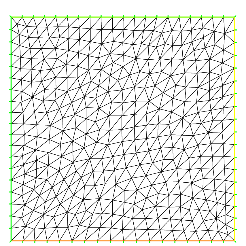
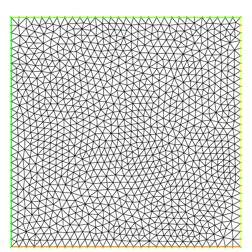
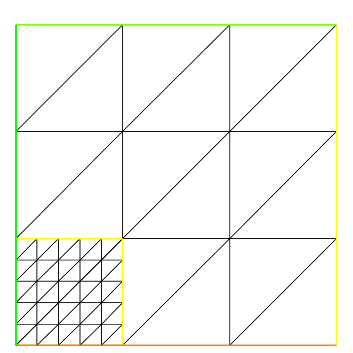
The command trunc
Two operators have been introduced to remove triangles from a mesh or to divide them.
Operator trunc has the following parameters:
boolean function to keep or remove elements
label=sets the label number of new boundary item, one by default.split=sets the level \(n\) of triangle splitting.Each triangle is split in \(n\times n\), one by default.
To create the mesh Th3 where all triangles of a mesh Th are split in \(3{\times}3\), just write:
1mesh Th3 = trunc(Th, 1, split=3);
The following example construct all “trunced” meshes to the support of the basic function of the space Vh (cf. abs(u)>0), split all the triangles in \(5{\times} 5\), and put a label number to \(2\) on a new boundary.
 1// Mesh
 2mesh Th = square(3, 3);
 3
 4// Fespace
 5fespace Vh(Th, P1);
 6Vh u=0;
 7
 8// Loop on all degrees of freedom
 9int n=u.n;
10for (int i = 0; i < n; i++){
11    u[][i] = 1; // The basis function i
12    plot(u, wait=true);
13    mesh Sh1 = trunc(Th, abs(u)>1.e-10, split=5, label=2);
14    plot(Th, Sh1, wait=true, ps="trunc"+i+".eps");
15    u[][i] = 0; // reset
16}
The command change
This command changes the label of elements and border elements of a mesh.
Changing the label of elements and border elements will be done using the keyword change.
The parameters for this command line are for two dimensional and three dimensional cases:
refe=is an array of integers to change the references on edgesreft=is an array of integers to change the references on triangleslabel=is an array of integers to change the 4 default label numbersregion=is an array of integers to change the default region numbersrenumv=is an array of integers, which explicitly gives the new numbering of vertices in the new mesh. By default, this numbering is that of the original meshrenumt=is an array of integers, which explicitly gives the new numbering of elements in the new mesh, according the new vertices numbering given byrenumv=. By default, this numbering is that of the original meshflabel=is an integer function given the new value of the labelfregion=is an integer function given the new value of the regionrmledges=is an integer to remove edges in the new mesh, following a labelrmInternalEdges=is a boolean, if equal to true to remove the internal edges. By default, the internal edges are stored
These vectors are composed of \(n_{l}\) successive pairs of numbers \(O,N\) where \(n_{l}\) is the number (label or region) that we want to change. For example, we have :
An application example is given here:
 1// Mesh
 2mesh Th1 = square(10, 10);
 3mesh Th2 = square(20, 10, [x+1, y]);
 4
 5int[int] r1=[2,0];
 6plot(Th1, wait=true);
 7
 8Th1 = change(Th1, label=r1); //change the label of Edges 2 in 0.
 9plot(Th1, wait=true);
10
11// boundary label: 1 -> 1 bottom, 2 -> 1 right, 3->1 top, 4->1 left boundary label is 1
12int[int] re=[1,1, 2,1, 3,1, 4,1]
13Th2=change(Th2,refe=re);
14plot(Th2,wait=1) ;
The command splitmesh
Another way to split mesh triangles is to use splitmesh, for example:
1// Mesh
2border a(t=0, 2*pi){x=cos(t); y=sin(t); label=1;}
3mesh Th = buildmesh(a(20));
4plot(Th, wait=true, ps="NotSplittedMesh.eps");
5
6// Splitmesh
7Th = splitmesh(Th, 1 + 5*(square(x-0.5) + y*y));
8plot(Th, wait=true, ps="SplittedMesh.eps");
Meshing Examples
Tip
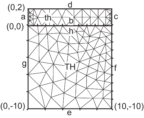
Two rectangles touching by a side
 1border a(t=0, 1){x=t; y=0;};
 2border b(t=0, 1){x=1; y=t;};
 3border c(t=1, 0){x=t; y=1;};
 4border d(t=1, 0){x=0; y=t;};
 5border c1(t=0, 1){x=t; y=1;};
 6border e(t=0, 0.2){x=1; y=1+t;};
 7border f(t=1, 0){x=t; y=1.2;};
 8border g(t=0.2, 0){x=0; y=1+t;};
 9int n=1;
10mesh th = buildmesh(a(10*n) + b(10*n) + c(10*n) + d(10*n));
11mesh TH = buildmesh(c1(10*n) + e(5*n) + f(10*n) + g(5*n));
12plot(th, TH, ps="TouchSide.esp");
Tip
NACA0012 Airfoil
1border upper(t=0, 1){x=t; y=0.17735*sqrt(t) - 0.075597*t - 0.212836*(t^2) + 0.17363*(t^3) - 0.06254*(t^4);}
2border lower(t=1, 0){x = t; y=-(0.17735*sqrt(t) -0.075597*t - 0.212836*(t^2) + 0.17363*(t^3) - 0.06254*(t^4));}
3border c(t=0, 2*pi){x=0.8*cos(t) + 0.5; y=0.8*sin(t);}
4mesh Th = buildmesh(c(30) + upper(35) + lower(35));
5plot(Th, ps="NACA0012.eps", bw=true);

Tip
Cardioid
1real b = 1, a = b;
2border C(t=0, 2*pi){x=(a+b)*cos(t)-b*cos((a+b)*t/b); y=(a+b)*sin(t)-b*sin((a+b)*t/b);}
3mesh Th = buildmesh(C(50));
4plot(Th, ps="Cardioid.eps", bw=true);

Tip
Cassini Egg
1border C(t=0, 2*pi) {x=(2*cos(2*t)+3)*cos(t); y=(2*cos(2*t)+3)*sin(t);}
2mesh Th = buildmesh(C(50));
3plot(Th, ps="Cassini.eps", bw=true);

Tip
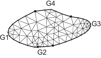
By cubic Bezier curve
 1// A cubic Bezier curve connecting two points with two control points
 2func real bzi(real p0, real p1, real q1, real q2, real t){
 3    return p0*(1-t)^3 + q1*3*(1-t)^2*t + q2*3*(1-t)*t^2 + p1*t^3;
 4}
 5
 6real[int] p00 = [0, 1], p01 = [0, -1], q00 = [-2, 0.1], q01 = [-2, -0.5];
 7real[int] p11 = [1,-0.9], q10 = [0.1, -0.95], q11=[0.5, -1];
 8real[int] p21 = [2, 0.7], q20 = [3, -0.4], q21 = [4, 0.5];
 9real[int] q30 = [0.5, 1.1], q31 = [1.5, 1.2];
10border G1(t=0, 1){
11    x=bzi(p00[0], p01[0], q00[0], q01[0], t);
12    y=bzi(p00[1], p01[1], q00[1], q01[1], t);
13}
14border G2(t=0, 1){
15    x=bzi(p01[0], p11[0], q10[0], q11[0], t);
16    y=bzi(p01[1], p11[1], q10[1], q11[1], t);
17}
18border G3(t=0, 1){
19    x=bzi(p11[0], p21[0], q20[0], q21[0], t);
20    y=bzi(p11[1], p21[1], q20[1], q21[1], t);
21}
22border G4(t=0, 1){
23    x=bzi(p21[0], p00[0], q30[0], q31[0], t);
24    y=bzi(p21[1], p00[1], q30[1], q31[1], t);
25}
26int m = 5;
27mesh Th = buildmesh(G1(2*m) + G2(m) + G3(3*m) + G4(m));
28plot(Th, ps="Bezier.eps", bw=true);
Tip
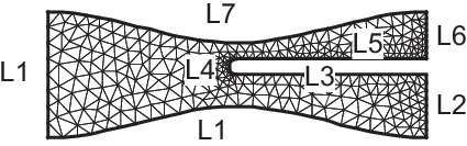
Section of Engine
 1real a = 6., b = 1., c = 0.5;
 2
 3border L1(t=0, 1){x=-a; y=1+b-2*(1+b)*t;}
 4border L2(t=0, 1){x=-a+2*a*t; y=-1-b*(x/a)*(x/a)*(3-2*abs(x)/a );}
 5border L3(t=0, 1){x=a; y=-1-b+(1+b)*t; }
 6border L4(t=0, 1){x=a-a*t; y=0;}
 7border L5(t=0, pi){x=-c*sin(t)/2; y=c/2-c*cos(t)/2;}
 8border L6(t=0, 1){x=a*t; y=c;}
 9border L7(t=0, 1){x=a; y=c+(1+b-c)*t;}
10border L8(t=0, 1){x=a-2*a*t; y=1+b*(x/a)*(x/a)*(3-2*abs(x)/a);}
11mesh Th = buildmesh(L1(8) + L2(26) + L3(8) + L4(20) + L5(8) + L6(30) + L7(8) + L8(30));
12plot(Th, ps="Engine.eps", bw=true);
Tip
Domain with U-shape channel
 1real d = 0.1; //width of U-shape
 2border L1(t=0, 1-d){x=-1; y=-d-t;}
 3border L2(t=0, 1-d){x=-1; y=1-t;}
 4border B(t=0, 2){x=-1+t; y=-1;}
 5border C1(t=0, 1){x=t-1; y=d;}
 6border C2(t=0, 2*d){x=0; y=d-t;}
 7border C3(t=0, 1){x=-t; y=-d;}
 8border R(t=0, 2){x=1; y=-1+t;}
 9border T(t=0, 2){x=1-t; y=1;}
10int n = 5;
11mesh Th = buildmesh(L1(n/2) + L2(n/2) + B(n) + C1(n) + C2(3) + C3(n) + R(n) + T(n));
12plot(Th, ps="U-shape.eps", bw=true);
Tip
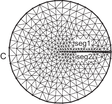
Domain with V-shape cut
 1real dAg = 0.02; //angle of V-shape
 2border C(t=dAg, 2*pi-dAg){x=cos(t); y=sin(t);};
 3real[int] pa(2), pb(2), pc(2);
 4pa[0] = cos(dAg);
 5pa[1] = sin(dAg);
 6pb[0] = cos(2*pi-dAg);
 7pb[1] = sin(2*pi-dAg);
 8pc[0] = 0;
 9pc[1] = 0;
10border seg1(t=0, 1){x=(1-t)*pb[0]+t*pc[0]; y=(1-t)*pb[1]+t*pc[1];};
11border seg2(t=0, 1){x=(1-t)*pc[0]+t*pa[0]; y=(1-t)*pc[1]+t*pa[1];};
12mesh Th = buildmesh(seg1(20) + C(40) + seg2(20));
13plot(Th, ps="V-shape.eps", bw=true);
Tip
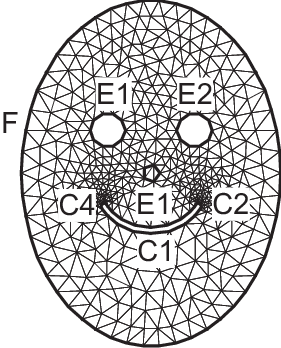
Smiling face
 1real d=0.1; int m = 5; real a = 1.5, b = 2, c = 0.7, e = 0.01;
 2
 3border F(t=0, 2*pi){x=a*cos(t); y=b*sin(t);}
 4border E1(t=0, 2*pi){x=0.2*cos(t)-0.5; y=0.2*sin(t)+0.5;}
 5border E2(t=0, 2*pi){x=0.2*cos(t)+0.5; y=0.2*sin(t)+0.5;}
 6func real st(real t){
 7    return sin(pi*t) - pi/2;
 8}
 9border C1(t=-0.5, 0.5){x=(1-d)*c*cos(st(t)); y=(1-d)*c*sin(st(t));}
10border C2(t=0, 1){x=((1-d)+d*t)*c*cos(st(0.5)); y=((1-d)+d*t)*c*sin(st(0.5));}
11border C3(t=0.5, -0.5){x=c*cos(st(t)); y=c*sin(st(t));}
12border C4(t=0, 1){x=(1-d*t)*c*cos(st(-0.5)); y=(1-d*t)*c*sin(st(-0.5));}
13border C0(t=0, 2*pi){x=0.1*cos(t); y=0.1*sin(t);}
14
15mesh Th=buildmesh(F(10*m) + C1(2*m) + C2(3) + C3(2*m) + C4(3)
16    + C0(m) + E1(-2*m) + E2(-2*m));
17plot(Th, ps="SmileFace.eps", bw=true);
Tip
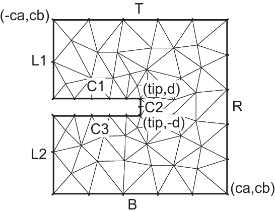
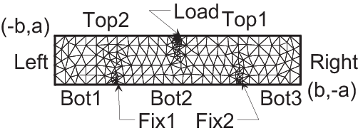
3 points bending
 1// Square for Three-Point Bend Specimens fixed on Fix1, Fix2
 2// It will be loaded on Load.
 3real a = 1, b = 5, c = 0.1;
 4int n = 5, m = b*n;
 5border Left(t=0, 2*a){x=-b; y=a-t;}
 6border Bot1(t=0, b/2-c){x=-b+t; y=-a;}
 7border Fix1(t=0, 2*c){x=-b/2-c+t; y=-a;}
 8border Bot2(t=0, b-2*c){x=-b/2+c+t; y=-a;}
 9border Fix2(t=0, 2*c){x=b/2-c+t; y=-a;}
10border Bot3(t=0, b/2-c){x=b/2+c+t; y=-a;}
11border Right(t=0, 2*a){x=b; y=-a+t;}
12border Top1(t=0, b-c){x=b-t; y=a;}
13border Load(t=0, 2*c){x=c-t; y=a;}
14border Top2(t=0, b-c){x=-c-t; y=a;}
15mesh Th = buildmesh(Left(n) + Bot1(m/4) + Fix1(5) + Bot2(m/2)
16    + Fix2(5) + Bot3(m/4) + Right(n) + Top1(m/2) + Load(10) + Top2(m/2));
17plot(Th, ps="ThreePoint.eps", bw=true);
The type mesh3 in 3 dimension
Note
Up to the version 3, FreeFEM allowed to consider a surface problem such as the PDE is treated like boundary conditions on the boundary domain (on triangles describing the boundary domain). With the version 4, in particular 4.2.1, a completed model for surface problem is possible, with the definition of a surface mesh and a surface problem with a variational form on domain ( with triangle elements) and application of boundary conditions on border domain (describing by edges). The keywords to define a surface mesh is meshS.
3d mesh generation
Note
For 3D mesh tools, put load "msh3" at the top of the .edp script.
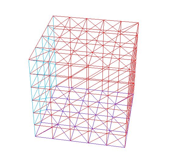
The command cube
The function cube like its 2d function square is a simple way to build cubic objects, it is contained in plugin msh3 (import with load "msh3").
The following code generates a \(3\times 4 \times 5\) grid in the unit cube \([0, 1]^3\).
1mesh3 Th = cube(3, 4, 5);
By default the labels are :
face \(y=0\),
face \(x=1\),
face \(y=1\),
face \(x=0\),
face \(z=0\),
face \(z=1\)
and the region number is \(0\).
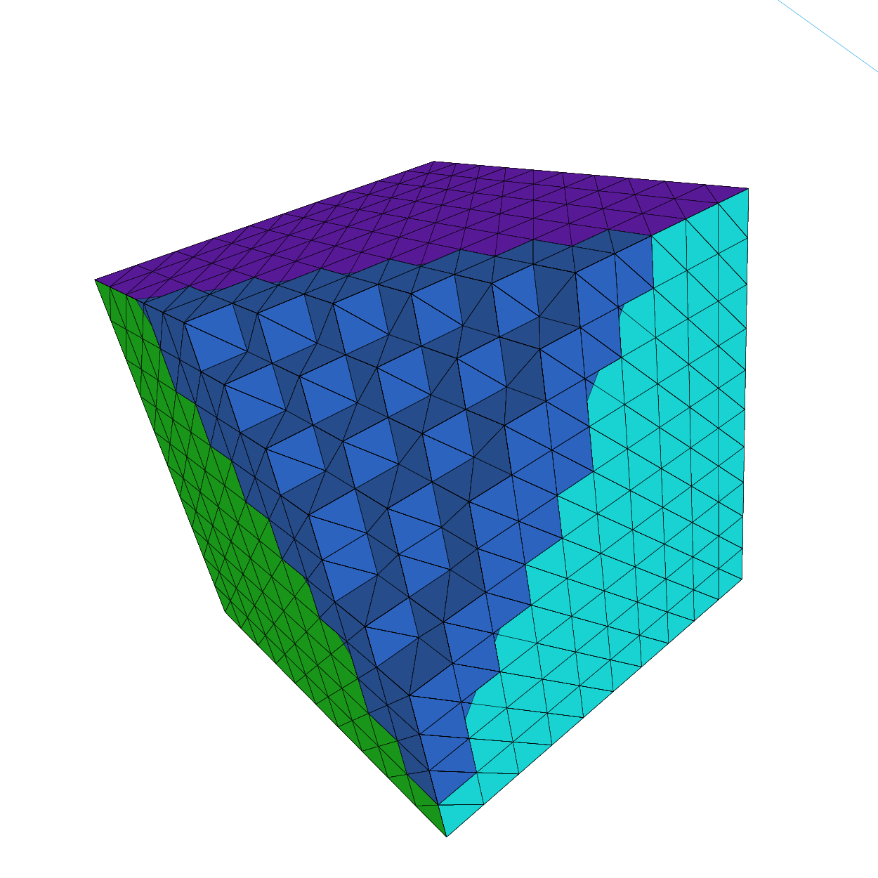
A full example of this function to build a mesh of cube \(]-1,1[^3\) with face label given by \((ix + 4*(iy+1) + 16*(iz+1))\) where \((ix, iy, iz)\) are the coordinates of the barycenter of the current face, is given below.
 1load "msh3"
 2
 3int[int] l6 = [37, 42, 45, 40, 25, 57];
 4int r11 = 11;
 5mesh3 Th = cube(4, 5, 6, [x*2-1, y*2-1, z*2-1], label=l6, flags =3, region=r11);
 6
 7cout << "Volume = " << Th.measure << ", border area = " << Th.bordermeasure << endl;
 8
 9int err = 0;
10for(int i = 0; i < 100; ++i){
11    real s = int2d(Th,i)(1.);
12    real sx = int2d(Th,i)(x);
13    real sy = int2d(Th,i)(y);
14    real sz = int2d(Th,i)(z);
15
16    if(s){
17        int ix = (sx/s+1.5);
18        int iy = (sy/s+1.5);
19        int iz = (sz/s+1.5);
20        int ii = (ix + 4*(iy+1) + 16*(iz+1) );
21        //value of ix,iy,iz => face min 0, face max 2, no face 1
22        cout << "Label = " << i << ", s = " << s << " " << ix << iy << iz << " : " << ii << endl;
23        if( i != ii ) err++;
24    }
25}
26real volr11 = int3d(Th,r11)(1.);
27cout << "Volume region = " << 11 << ": " << volr11 << endl;
28if((volr11 - Th.measure )>1e-8) err++;
29plot(Th, fill=false);
30cout << "Nb err = " << err << endl;
31assert(err==0);
The output of this script is:
 1Enter: BuildCube: 3
 2  kind = 3 n tet Cube = 6 / n slip 6 19
 3Cube  nv=210 nt=720 nbe=296
 4Out:  BuildCube
 5Volume = 8, border area = 24
 6Label = 25, s = 4 110 : 25
 7Label = 37, s = 4 101 : 37
 8Label = 40, s = 4 011 : 40
 9Label = 42, s = 4 211 : 42
10Label = 45, s = 4 121 : 45
11Label = 57, s = 4 112 : 57
12Volume region = 11: 8
13Nb err = 0
The command buildlayers
This mesh is obtained by extending a two dimensional mesh in the \(z\)-axis.
The domain \(\Omega_{3d}\) defined by the layer mesh is equal to \(\Omega_{3d} = \Omega_{2d} \times [zmin, zmax]\) where \(\Omega_{2d}\) is the domain defined by the two dimensional meshes. \(zmin\) and \(zmax\) are functions of \(\Omega_{2d}\) in \(\R\) that defines respectively the lower surface and upper surface of \(\Omega_{3d}\).

For a vertex of a two dimensional mesh \(V_{i}^{2d} = (x_{i},y_{i})\), we introduce the number of associated vertices in the \(z-\)axis \(M_{i}+1\).
We denote by \(M\) the maximum of \(M_{i}\) over the vertices of the two dimensional mesh. This value is called the number of layers (if \(\forall i, \; M_{i}=M\) then there are \(M\) layers in the mesh of \(\Omega_{3d}\)). \(V_{i}^{2d}\) generated \(M+1\) vertices which are defined by:
where \((z_{i,j})_{j=0,\ldots,M}\) are the \(M+1\) equidistant points on the interval \([zmin( V_{i}^{2d} ), zmax( V_{i}^{2d})]\):
The function \(\theta_{i}\), defined on \([zmin( V_{i}^{2d} ), zmax( V_{i}^{2d} )]\), is given by:
with \((\theta_{i,j})_{j=0,\ldots,M_{i}}\) are the \(M_{i}+1\) equidistant points on the interval \([zmin( V_{i}^{2d} ), zmax( V_{i}^{2d} )]\).
Set a triangle \(K=(V_{i1}^{2d}\), \(V_{i2}^{2d}\), \(V_{i3}^{2d})\) of the two dimensional mesh. \(K\) is associated with a triangle on the upper surface (resp. on the lower surface) of layer mesh:
\(( V_{i1,M}^{3d}, V_{i2,M}^{3d}, V_{i3,M}^{3d} )\) (resp. \(( V_{i1,0}^{3d}, V_{i2,0}^{3d}, V_{i3,0}^{3d})\)).
Also \(K\) is associated with \(M\) volume prismatic elements which are defined by:
Theses volume elements can have some merged point:
0 merged point : prism
1 merged points : pyramid
2 merged points : tetrahedra
3 merged points : no elements
The elements with merged points are called degenerate elements. To obtain a mesh with tetrahedra, we decompose the pyramid into two tetrahedra and the prism into three tetrahedra. These tetrahedra are obtained by cutting the quadrilateral face of pyramid and prism with the diagonal which have the vertex with the maximum index (see [HECHT1992] for the reason of this choice).
The triangles on the middle surface obtained with the decomposition of the volume prismatic elements are the triangles generated by the edges on the border of the two dimensional mesh. The label of triangles on the border elements and tetrahedra are defined with the label of these associated elements.
The arguments of buildlayers is a two dimensional mesh and the number of layers \(M\).
The parameters of this command are:
zbound=\([zmin,zmax]\) where \(zmin\) and \(zmax\) are functions expression.Theses functions define the lower surface mesh and upper mesh of surface mesh.
coef=A function expression between [0,1].This parameter is used to introduce degenerate element in mesh.
The number of associated points or vertex \(V_{i}^{2d}\) is the integer part of \(coef(V_{i}^{2d}) M\).
region=This vector is used to initialize the region of tetrahedra.This vector contains successive pairs of the 2d region number at index \(2i\) and the corresponding 3d region number at index \(2i+1\), like change.
labelmid=This vector is used to initialize the 3d labels number of the vertical face or mid face from the 2d label number.This vector contains successive pairs of the 2d label number at index \(2i\) and the corresponding 3d label number at index \(2i+1\), like change.
labelup=This vector is used to initialize the 3d label numbers of the upper/top face from the 2d region number.This vector contains successive pairs of the 2d region number at index \(2i\) and the corresponding 3d label number at index \(2i+1\), like change.
labeldown=Same as the previous case but for the lower/down face label.
Moreover, we also add post processing parameters that allow to moving the mesh.
These parameters correspond to parameters transfo, facemerge and ptmerge of the command line movemesh.
The vector region, labelmid, labelup and labeldown These vectors are composed of \(n_{l}\) successive pairs of number \(O_i,N_l\) where \(n_{l}\) is the number (label or region) that we want to get.
An example of this command is given in the Build layer mesh example.
Tip
Cube
 1//Cube.idp
 2load "medit"
 3load "msh3"
 4
 5func mesh3 Cube (int[int] &NN, real[int, int] &BB, int[int, int] &L){
 6    real x0 = BB(0,0), x1 = BB(0,1);
 7    real y0 = BB(1,0), y1 = BB(1,1);
 8    real z0 = BB(2,0), z1 = BB(2,1);
 9
10    int nx = NN[0], ny = NN[1], nz = NN[2];
11
12    // 2D mesh
13    mesh Thx = square(nx, ny, [x0+(x1-x0)*x, y0+(y1-y0)*y]);
14
15    // 3D mesh
16    int[int] rup = [0, L(2,1)], rdown=[0, L(2,0)];
17    int[int] rmid=[1, L(1,0), 2, L(0,1), 3, L(1,1), 4, L(0,0)];
18    mesh3 Th = buildlayers(Thx, nz, zbound=[z0,z1],
19    labelmid=rmid, labelup = rup, labeldown = rdown);
20
21    return Th;
22}
Tip
Unit cube
1include "Cube.idp"
2
3int[int] NN = [10,10,10]; //the number of step in each direction
4real [int, int] BB = [[0,1],[0,1],[0,1]]; //the bounding box
5int [int, int] L = [[1,2],[3,4],[5,6]]; //the label of the 6 face left,right, front, back, down, right
6mesh3 Th = Cube(NN, BB, L);
7medit("Th", Th);
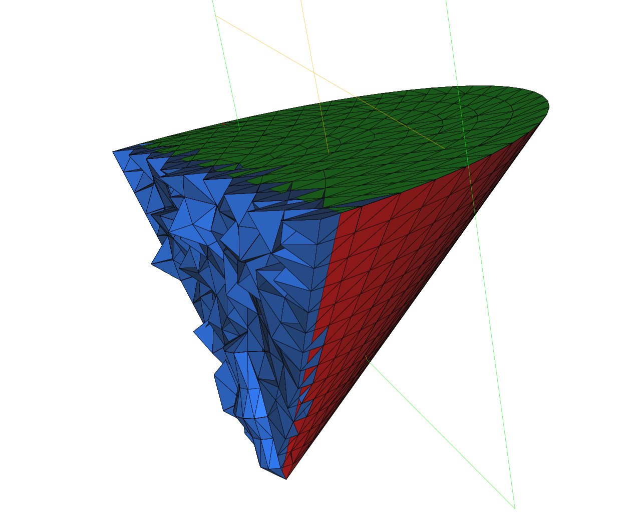
Tip
Cone
An axisymtric mesh on a triangle with degenerateness
 1load "msh3"
 2load "medit"
 3
 4// Parameters
 5real RR = 1;
 6real HH = 1;
 7
 8int nn=10;
 9
10// 2D mesh
11border Taxe(t=0, HH){x=t; y=0; label=0;}
12border Hypo(t=1, 0){x=HH*t; y=RR*t; label=1;}
13border Vert(t=0, RR){x=HH; y=t; label=2;}
14mesh Th2 = buildmesh(Taxe(HH*nn) + Hypo(sqrt(HH*HH+RR*RR)*nn) + Vert(RR*nn));
15plot(Th2, wait=true);
16
17// 3D mesh
18real h = 1./nn;
19int MaxLayersT = (int(2*pi*RR/h)/4)*4;//number of layers
20real zminT = 0;
21real zmaxT = 2*pi; //height 2*pi
22func fx = y*cos(z);
23func fy = y*sin(z);
24func fz = x;
25int[int] r1T = [0,0], r2T = [0,0,2,2], r4T = [0,2];
26//trick function:
27//The function defined the proportion
28//of number layer close to axis with reference MaxLayersT
29func deg = max(.01, y/max(x/HH, 0.4)/RR);
30mesh3 Th3T = buildlayers(Th2, coef=deg, MaxLayersT,
31    zbound=[zminT, zmaxT], transfo=[fx, fy, fz],
32    facemerge=0, region=r1T, labelmid=r2T);
33medit("cone", Th3T);
Tip
Buildlayer mesh
 1load "msh3"
 2load "TetGen"
 3load "medit"
 4
 5// Parameters
 6int C1 = 99;
 7int C2 = 98;
 8
 9// 2D mesh
10border C01(t=0, pi){x=t; y=0; label=1;}
11border C02(t=0, 2*pi){ x=pi; y=t; label=1;}
12border C03(t=0, pi){ x=pi-t; y=2*pi; label=1;}
13border C04(t=0, 2*pi){ x=0; y=2*pi-t; label=1;}
14
15border C11(t=0, 0.7){x=0.5+t; y=2.5; label=C1;}
16border C12(t=0, 2){x=1.2; y=2.5+t; label=C1;}
17border C13(t=0, 0.7){x=1.2-t; y=4.5; label=C1;}
18border C14(t=0, 2){x=0.5; y=4.5-t; label=C1;}
19
20border C21(t=0, 0.7){x=2.3+t; y=2.5; label=C2;}
21border C22(t=0, 2){x=3; y=2.5+t; label=C2;}
22border C23(t=0, 0.7){x=3-t; y=4.5; label=C2;}
23border C24(t=0, 2){x=2.3; y=4.5-t; label=C2;}
24
25mesh Th = buildmesh(C01(10) + C02(10) + C03(10) + C04(10)
26    + C11(5) + C12(5) + C13(5) + C14(5)
27    + C21(-5) + C22(-5) + C23(-5) + C24(-5));
28
29mesh Ths = buildmesh(C01(10) + C02(10) + C03(10) + C04(10)
30    + C11(5) + C12(5) + C13(5) + C14(5));
31
32// Construction of a box with one hole and two regions
33func zmin = 0.;
34func zmax = 1.;
35int MaxLayer = 10;
36
37func XX = x*cos(y);
38func YY = x*sin(y);
39func ZZ = z;
40
41int[int] r1 = [0, 41], r2 = [98, 98, 99, 99, 1, 56];
42int[int] r3 = [4, 12];  //the triangles of uppper surface mesh
43                        //generated by the triangle in the 2D region
44                        //of mesh Th of label 4 as label 12
45int[int] r4 = [4, 45];  //the triangles of lower surface mesh
46                        //generated by the triangle in the 2D region
47                        //of mesh Th of label 4 as label 45.
48
49mesh3 Th3 = buildlayers(Th, MaxLayer, zbound=[zmin, zmax], region=r1,
50    labelmid=r2, labelup=r3, labeldown=r4);
51    medit("box 2 regions 1 hole", Th3);
52
53// Construction of a sphere with TetGen
54func XX1 = cos(y)*sin(x);
55func YY1 = sin(y)*sin(x);
56func ZZ1 = cos(x);
57
58real[int] domain = [0., 0., 0., 0, 0.001];
59string test = "paACQ";
60cout << "test = " << test << endl;
61mesh3 Th3sph = tetgtransfo(Ths, transfo=[XX1, YY1, ZZ1],
62    switch=test, nbofregions=1, regionlist=domain);
63medit("sphere 2 regions", Th3sph);
Remeshing
Note
if an operation on a mesh3 is performed then the same operation is applyed on its surface part (its meshS associated)
The command change
This command changes the label of elements and border elements of a mesh. It’s the equivalent command in 2d mesh case.
Changing the label of elements and border elements will be done using the keyword change.
The parameters for this command line are for two dimensional and three dimensional cases:
reftet=is a vector of integer that contains successive pairs of the old label number to the new label number.refface=is a vector of integer that contains successive pairs of the old region number to new region number.flabel=is an integer function given the new value of the label.fregion=is an integer function given the new value of the region.rmInternalFaces=is a boolean, equal true to remove the internal faces.rmlfaces=is a vector of integer, where triangle’s label given are remove of the mesh
These vectors are composed of \(n_{l}\) successive pairs of numbers \(O,N\) where \(n_{l}\) is the number (label or region) that we want to change. For example, we have:
An example of use:
 1// Mesh
 2mesh3 Th1 = cube(10, 10);
 3mesh3 Th2 = cube(20, 10, [x+1, y,z]);
 4
 5int[int] r1=[2,0];
 6plot(Th1, wait=true);
 7
 8Th1 = change(Th1, label=r1); //change the label of Edges 2 in 0.
 9plot(Th1, wait=true);
10
11// boundary label: 1 -> 1 bottom, 2 -> 1 right, 3->1 top, 4->1 left boundary label is 1
12int[int] re=[1,1, 2,1, 3,1, 4,1]
13Th2=change(Th2,refe=re);
14plot(Th2,wait=1) ;
The command trunc
This operator have been introduce to remove a piece of mesh or/and split all element or for a particular label element
The three named parameter
- boolean function to keep or remove elements
- split= sets the level n of triangle splitting. each triangle is splitted in n × n ( one by default)
- freefem:label= sets the label number of new boundary item (1 by default)
An example of use
1load "msh3"
2load "medit"
3int nn=8;
4mesh3 Th=cube(nn,nn,nn);
5//  remove the small cube $]1/2,1[^2$
6Th= trunc(Th,((x<0.5) |(y< 0.5)| (z<0.5)), split=3, label=3);
7medit("cube",Th);
The command movemesh
3D meshes can be translated, rotated, and deformed using the command line movemesh as in the 2D case (see section movemesh).
If \(\Omega\) is tetrahedrized as \(T_{h}(\Omega)\), and \(\Phi(x,y)=(\Phi1(x,y,z), \Phi2(x,y,z), \Phi3(x,y,z))\) is the transformation vector then \(\Phi(T_{h})\) is obtained by:
1mesh3 Th = movemesh(Th, [Phi1, Phi2, Phi3], ...);
2mesh3 Th = movemesh3(Th, transfo=[Phi1, Phi2, Phi3], ...);  (syntax with transfo=)
The parameters of movemesh in three dimensions are:
transfo=sets the geometric transformation \(\Phi(x,y)=(\Phi1(x,y,z), \Phi2(x,y,z), \Phi3(x,y,z))\)region=sets the integer labels of the tetrahedra.0 by default.
label=sets the labels of the border faces.This parameter is initialized as the label for the keyword change.
facemerge=An integer expression.When you transform a mesh, some faces can be merged. This parameter equals to one if the merges’ faces is considered. Otherwise it equals to zero. By default, this parameter is equal to 1.
ptmerge =A real expression.When you transform a mesh, some points can be merged. This parameter is the criteria to define two merging points. By default, we use
\[ptmerge \: = \: 1e-7 \: \:Vol( B ),\]
where \(B\) is the smallest axis parallel boxes containing the discretion domain of \(\Omega\) and \(Vol(B)\) is the volume of this box.
orientation =An integer expression equal 1, give the oientation of the triangulation, elements must be in the reference orientation (counter clock wise) equal -1 reverse the orientation of the tetrahedra
Note
The orientation of tetrahedra are checked by the positivity of its area and automatically corrected during the building of the adjacency.
An example of this command can be found in the Poisson’s equation 3D example.
 1load "medit"
 2include "cube.idp"
 3int[int]  Nxyz=[20,5,5];
 4real [int,int]  Bxyz=[[0.,5.],[0.,1.],[0.,1.]];
 5int [int,int]  Lxyz=[[1,2],[2,2],[2,2]];
 6real E = 21.5e4;
 7real sigma = 0.29;
 8real mu = E/(2*(1+sigma));
 9real lambda = E*sigma/((1+sigma)*(1-2*sigma));
10real gravity = -0.05;
11real sqrt2=sqrt(2.);
12
13mesh3 Th=Cube(Nxyz,Bxyz,Lxyz);
14fespace Vh(Th,[P1,P1,P1]);
15Vh [u1,u2,u3], [v1,v2,v3];
16
17macro epsilon(u1,u2,u3)  [dx(u1),dy(u2),dz(u3),(dz(u2)+dy(u3))/sqrt2,(dz(u1)+dx(u3))/sqrt2,(dy(u1)+dx(u2))/sqrt2] // EOM
18macro div(u1,u2,u3) ( dx(u1)+dy(u2)+dz(u3) ) // EOM
19
20solve Lame([u1,u2,u3],[v1,v2,v3])=
21  int3d(Th)(
22            lambda*div(u1,u2,u3)*div(v1,v2,v3)
23            +2.*mu*( epsilon(u1,u2,u3)'*epsilon(v1,v2,v3) )
24              )
25  - int3d(Th) (gravity*v3)
26  + on(1,u1=0,u2=0,u3=0);
27
28real dmax= u1[].max;
29real coef= 0.1/dmax;
30
31int[int] ref2=[1,0,2,0]; // array
32mesh3 Thm=movemesh(Th,[x+u1*coef,y+u2*coef,z+u3*coef],label=ref2);
33// mesh3 Thm=movemesh3(Th,transfo=[x+u1*coef,y+u2*coef,z+u3*coef],label=ref2); older syntax
34Thm=change(Thm,label=ref2);
35plot(Th,Thm, wait=1,cmm="coef  amplification = "+coef );
movemesh doesn’t use the prefix tranfo= [.,.,.], the geometric transformation is directly given by [.,.,.] in the arguments list
The command extract
This command offers the possibility to extract a boundary part of a mesh3
refface, is a vector of integer that contains a list of triangle face references, where the extract function must be apply.label, is a vector of integer that contains a list of tetrahedra label
1load"msh3"
2int nn = 30;
3int[int] labs = [1, 2, 2, 1, 1, 2]; // Label numbering
4mesh3 Th = cube(nn, nn, nn, label=labs);
5// extract the surface (boundary) of the cube
6int[int] llabs = [1, 2];
7meshS ThS = extract(Th,label=llabs);
The command buildSurface
This new function allows to build the surface mesh of a volume mesh, under the condition the surface is the boundary of the volume. By definition, a mesh3 is defined by a list of vertices, tetrahedron elements and triangle border elements. buildSurface function create the meshS corresponding, given the list vertices which are on the border domain, the triangle elements and build the list of edges. Remark, for a closed surface mesh, the edges list is empty.
The command movemesh23
A simple method to tranform a 2D mesh in 3D Surface mesh. The principe is to project a two dimensional domain in a three dimensional space, 2d surface in the (x,y,z)-space to create a surface mesh 3D, meshS.
Warning
Since the release 4.2.1, the FreeFEM function movemesh23 returns a meshS type.
This corresponds to translate, rotate or deforme the domain by a displacement vector of this form \(\mathbf{\Phi(x,y)} = (\Phi1(x,y), \Phi2(x,y), \Phi3(x,y))\).
The result of moving a two dimensional mesh Th2 by this three dimensional displacement is obtained using:
1**meshS** Th3 = movemesh23(Th2, transfo=[Phi(1), Phi(2), Phi(3)]);
The parameters of this command line are:
transfo=[\(\Phi 1\), \(\Phi 2\), \(\Phi 3\)] sets the displacement vector of transformation \(\mathbf{\Phi(x,y)} = [\Phi1(x,y), \Phi2(x,y), \Phi3(x,y)]\).label=sets an integer label of triangles.orientation=sets an integer orientation to give the global orientation of the surface of mesh. Equal 1, give a triangulation in the reference orientation (counter clock wise) equal -1 reverse the orientation of the trianglesptmerge=A real expression.When you transform a mesh, some points can be merged. This parameter is the criteria to define two merging points. By default, we use
\[ptmerge \: = \: 1e-7 \: \:Vol( B ),\]
where \(B\) is the smallest axis, parallel boxes containing the discretized domain of \(\Omega\) and \(Vol(B)\) is the volume of this box.
We can do a “gluing” of surface meshes using the process given in Change section.
An example to obtain a three dimensional mesh using the command line tetg and movemesh23 is given below.
 1load "msh3"
 2load "tetgen"
 3
 4// Parameters
 5real x10 = 1.;
 6real x11 = 2.;
 7real y10 = 0.;
 8real y11 = 2.*pi;
 9
10func ZZ1min = 0;
11func ZZ1max = 1.5;
12func XX1 = x;
13func YY1 = y;
14
15real x20 = 1.;
16real x21 = 2.;
17real y20=0.;
18real y21=1.5;
19
20func ZZ2 = y;
21func XX2 = x;
22func YY2min = 0.;
23func YY2max = 2*pi;
24
25real x30=0.;
26real x31=2*pi;
27real y30=0.;
28real y31=1.5;
29
30func XX3min = 1.;
31func XX3max = 2.;
32func YY3 = x;
33func ZZ3 = y;
34
35// Mesh
36mesh Thsq1 = square(5, 35, [x10+(x11-x10)*x, y10+(y11-y10)*y]);
37mesh Thsq2 = square(5, 8, [x20+(x21-x20)*x, y20+(y21-y20)*y]);
38mesh Thsq3 = square(35, 8, [x30+(x31-x30)*x, y30+(y31-y30)*y]);
39
40// Mesh 2D to 3D surface
41meshS Th31h = movemesh23(Thsq1, transfo=[XX1, YY1, ZZ1max], orientation=1);
42meshS Th31b = movemesh23(Thsq1, transfo=[XX1, YY1, ZZ1min], orientation=-1);
43
44meshS Th32h = movemesh23(Thsq2, transfo=[XX2, YY2max, ZZ2], orientation=-1);
45meshS Th32b = movemesh23(Thsq2, transfo=[XX2, YY2min, ZZ2], orientation=1);
46
47meshS Th33h = movemesh23(Thsq3, transfo=[XX3max, YY3, ZZ3], orientation=1);
48meshS Th33b = movemesh23(Thsq3, transfo=[XX3min, YY3, ZZ3], orientation=-1);
49
50// Gluing surfaces
51meshS Th33 = Th31h + Th31b + Th32h + Th32b + Th33h + Th33b;
52plot(Th33, cmm="Th33");
53
54// Tetrahelize the interior of the cube with TetGen
55real[int] domain =[1.5, pi, 0.75, 145, 0.0025];
56meshS Thfinal = tetg(Th33, switch="paAAQY", regionlist=domain);
57plot(Thfinal, cmm="Thfinal");
58
59// Build a mesh of a half cylindrical shell of interior radius 1, and exterior radius 2 and a height of 1.5
60func mv2x = x*cos(y);
61func mv2y = x*sin(y);
62func mv2z = z;
63meshS Thmv2 = movemesh(Thfinal, transfo=[mv2x, mv2y, mv2z], facemerge=0);
64plot(Thmv2, cmm="Thmv2");
3d Meshing examples
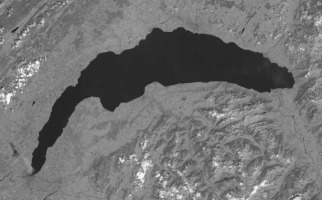
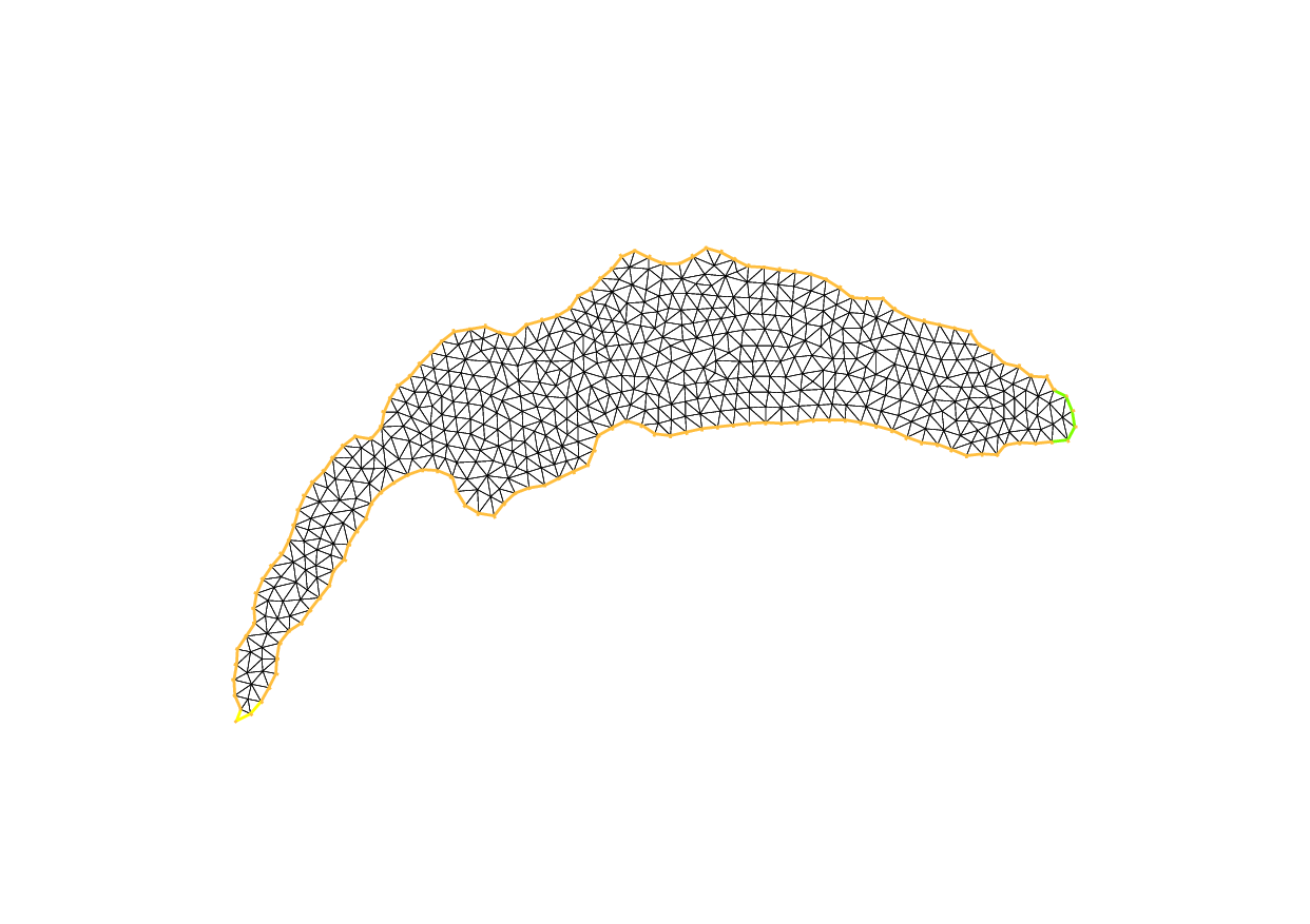
Tip
Lake
 1load "msh3"
 2load "medit"
 3
 4// Parameters
 5int nn = 5;
 6
 7// 2D mesh
 8border cc(t=0, 2*pi){x=cos(t); y=sin(t); label=1;}
 9mesh Th2 = buildmesh(cc(100));
10
11// 3D mesh
12int[int] rup = [0, 2], rlow = [0, 1];
13int[int] rmid = [1, 1, 2, 1, 3, 1, 4, 1];
14func zmin = 2-sqrt(4-(x*x+y*y));
15func zmax = 2-sqrt(3.);
16
17mesh3 Th = buildlayers(Th2, nn,
18    coef=max((zmax-zmin)/zmax, 1./nn),
19    zbound=[zmin,zmax],
20    labelmid=rmid,
21    labelup=rup,
22    labeldown=rlow);
23
24medit("Th", Th);
Tip
Hole region
 1load "msh3"
 2load "TetGen"
 3load "medit"
 4
 5// 2D mesh
 6mesh Th = square(10, 20, [x*pi-pi/2, 2*y*pi]); // ]-pi/2, pi/2[X]0,2pi[
 7
 8// 3D mesh
 9//parametrization of a sphere
10func f1 = cos(x)*cos(y);
11func f2 = cos(x)*sin(y);
12func f3 = sin(x);
13//partial derivative of the parametrization
14func f1x = sin(x)*cos(y);
15func f1y = -cos(x)*sin(y);
16func f2x = -sin(x)*sin(y);
17func f2y = cos(x)*cos(y);
18func f3x = cos(x);
19func f3y = 0;
20//M = DF^t DF
21func m11 = f1x^2 + f2x^2 + f3x^2;
22func m21 = f1x*f1y + f2x*f2y + f3x*f3y;
23func m22 = f1y^2 + f2y^2 + f3y^2;
24
25func perio = [[4, y], [2, y], [1, x], [3, x]];
26real hh = 0.1;
27real vv = 1/square(hh);
28verbosity = 2;
29Th = adaptmesh(Th, m11*vv, m21*vv, m22*vv, IsMetric=1, periodic=perio);
30Th = adaptmesh(Th, m11*vv, m21*vv, m22*vv, IsMetric=1, periodic=perio);
31plot(Th, wait=true);
32
33//construction of the surface of spheres
34real Rmin = 1.;
35func f1min = Rmin*f1;
36func f2min = Rmin*f2;
37func f3min = Rmin*f3;
38
39meshS ThSsph = movemesh23(Th, transfo=[f1min, f2min, f3min]);
40
41real Rmax = 2.;
42func f1max = Rmax*f1;
43func f2max = Rmax*f2;
44func f3max = Rmax*f3;
45
46meshS ThSsph2 = movemesh23(Th, transfo=[f1max, f2max, f3max]);
47
48//gluing meshes
49meshS ThS = ThSsph + ThSsph2;
50
51cout << " TetGen call without hole " << endl;
52real[int] domain2 = [1.5, 0., 0., 145, 0.001, 0.5, 0., 0., 18, 0.001];
53mesh3 Th3fin = tetg(ThS, switch="paAAQYY", nbofregions=2, regionlist=domain2);
54medit("Sphere with two regions", Th3fin);
55
56cout << " TetGen call with hole " << endl;
57real[int] hole = [0.,0.,0.];
58real[int] domain = [1.5, 0., 0., 53, 0.001];
59mesh3 Th3finhole = tetg(ThS, switch="paAAQYY",
60    nbofholes=1, holelist=hole, nbofregions=1, regionlist=domain);
61medit("Sphere with a hole", Th3finhole);
Tip
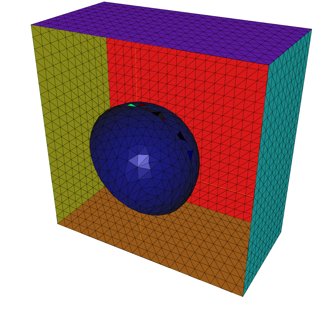
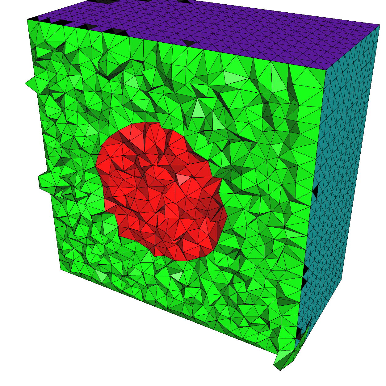
Build a 3d mesh of a cube with a balloon
 1load "msh3"
 2load "TetGen"
 3load "medit"
 4include "MeshSurface.idp"
 5
 6// Parameters
 7real hs = 0.1; //mesh size on sphere
 8int[int] N = [20, 20, 20];
 9real [int,int] B = [[-1, 1], [-1, 1], [-1, 1]];
10int [int,int] L = [[1, 2], [3, 4], [5, 6]];
11
12// Meshes
13meshS ThH = SurfaceHex(N, B, L, 1);
14meshS ThS = Sphere(0.5, hs, 7, 1);
15
16meshS ThHS = ThH + ThS;
17medit("Hex-Sphere", ThHS);
18
19real voltet = (hs^3)/6.;
20cout << "voltet = " << voltet << endl;
21real[int] domain = [0, 0, 0, 1, voltet, 0, 0, 0.7, 2, voltet];
22mesh3 Th = tetg(ThHS, switch="pqaAAYYQ", nbofregions=2, regionlist=domain);
23medit("Cube with ball", Th);
The type meshS in 3 dimension
Warning
Since the release 4.2.1, the surface mesh3 object (list of vertices and border elements, without tetahedra elements) is remplaced by meshS type.
Commands for 3d surface mesh generation
The command square3
The function square3 like the function square in 2d is the simple way to a build the unit square plan in the space \(\mathbb{R^3}\).
To use this command, it is necessary to load the pluging msh3 (need load "msh3").
A square in 3d consists in building a 2d square which is projected from \(\mathbb{R^2}\) to \(\mathbb{R^3}\).
The parameters of this command line are:
n,m generates a n×m grid in the unit square
[.,.,.]is [ \(\Phi 1\), \(\Phi 2\), \(\Phi 3\) ] is the geometric transformation from \(\mathbb{R^2}\) to \(\mathbb{R^3}\). By default, [ \(\Phi 1\), \(\Phi 2\), \(\Phi 3\) ] = [x,y,0]
orientation=equal 1, gives the orientation of the triangulation, elements are in the reference orientation (counter clock wise) equal -1 reverse the orientation of the triangles it’s the global orientation of the surface 1 extern (-1 intern)
 1     real R = 3, r=1;
 2     real h = 0.2; //
 3     int nx = R*2*pi/h;
 4     int ny = r*2*pi/h;
 5     func torex= (R+r*cos(y*pi*2))*cos(x*pi*2);
 6     func torey= (R+r*cos(y*pi*2))*sin(x*pi*2);
 7     func torez= r*sin(y*pi*2);
 8
 9
10     meshS ThS=square3(nx,ny,[torex,torey,torez],orientation=-1) ;
The following code generates a \(3\times 4 \times 5\) grid in the unit cube \([0, 1]^3\) with a clock wise triangulation.
surface mesh builders
Adding at the top of a FreeFEM script include "MeshSurface.idp", constructors of sphere, ellipsoid, surface mesh of a 3d box are available.
SurfaceHex(N, B, L, orient)
this operator allows to build the surface mesh of a 3d box
int[int] N=[nx,ny,nz]; // the number of seg in the 3 direction
real [int,int] B=[[xmin,xmax],[ymin,ymax],[zmin,zmax]]; // bounding bax
int [int,int] L=[[1,2],[3,4],[5,6]]; // the label of the 6 face left,right, front, back, down, right
orient the global orientation of the surface 1 extern (-1 intern),
returns a
meshStype
Ellipsoide (RX, RY, RZ, h, L, OX, OY, OZ, orient)
h is the mesh size
L is the label
orient the global orientation of the surface 1 extern (-1 intern)
OX, OY, OZ are real numbers to give the Ellipsoide center ( optinal, by default is (0,0,0) )
where RX, RY, RZ are real numbers such as the parametric equations of the ellipsoid is:
returns a
meshStype\[\forall u \in [- \frac{\pi}{2},\frac{\pi}{2} [ \text{ and } v \in [0, 2 \pi], \vectthree{x=\text{Rx } cos(u)cos(v) + \text{Ox }}{y=\text{Ry } cos(u)sin(v) + \text{Oy }}{z = \text{Rz } sin(v) + \text{Oz } }\]
Sphere(R, h, L, OX, OY, OZ, orient)
where R is the raduis of the sphere,
OX, OY, OZ are real numbers to give the Ellipsoide center ( optinal, by default is (0,0,0) )
h is the mesh size of the shpere
L is the label the the sphere
orient the global orientation of the surface 1 extern (-1 intern)
returns a
meshStype
 1func meshS SurfaceHex(int[int] & N,real[int,int] &B ,int[int,int] & L,int orientation){
 2    real x0=B(0,0),x1=B(0,1);
 3    real y0=B(1,0),y1=B(1,1);
 4    real z0=B(2,0),z1=B(2,1);
 5
 6    int nx=N[0],ny=N[1],nz=N[2];
 7
 8    mesh Thx = square(ny,nz,[y0+(y1-y0)*x,z0+(z1-z0)*y]);
 9    mesh Thy = square(nx,nz,[x0+(x1-x0)*x,z0+(z1-z0)*y]);
10    mesh Thz = square(nx,ny,[x0+(x1-x0)*x,y0+(y1-y0)*y]);
11
12    int[int] refx=[0,L(0,0)],refX=[0,L(0,1)];   //  Xmin, Ymax faces labels renumbering
13    int[int] refy=[0,L(1,0)],refY=[0,L(1,1)];   //  Ymin, Ymax faces labesl renumbering
14    int[int] refz=[0,L(2,0)],refZ=[0,L(2,1)];   //  Zmin, Zmax faces labels renumbering
15
16    meshS Thx0 = movemesh23(Thx,transfo=[x0,x,y],orientation=-orientation,label=refx);
17    meshS Thx1 = movemesh23(Thx,transfo=[x1,x,y],orientation=+orientation,label=refX);
18    meshS Thy0 = movemesh23(Thy,transfo=[x,y0,y],orientation=+orientation,label=refy);
19    meshS Thy1 = movemesh23(Thy,transfo=[x,y1,y],orientation=-orientation,label=refY);
20    meshS Thz0 = movemesh23(Thz,transfo=[x,y,z0],orientation=-orientation,label=refz);
21    meshS Thz1 = movemesh23(Thz,transfo=[x,y,z1],orientation=+orientation,label=refZ);
22    meshS Th= Thx0+Thx1+Thy0+Thy1+Thz0+Thz1;
23
24 return Th;
25 }
26
27 func meshS Ellipsoide (real RX,real RY,real RZ,real h,int L,real Ox,real Oy,real Oz,int orientation) {
28    mesh  Th=square(10,20,[x*pi-pi/2,2*y*pi]);  //  $]\frac{-pi}{2},frac{-pi}{2}[\times]0,2\pi[ $
29    //  a parametrization of a sphere
30    func f1 =RX*cos(x)*cos(y);
31    func f2 =RY*cos(x)*sin(y);
32    func f3 =RZ*sin(x);
33        //    partiel derivative
34    func f1x= -RX*sin(x)*cos(y);
35    func f1y= -RX*cos(x)*sin(y);
36    func f2x= -RY*sin(x)*sin(y);
37    func f2y= +RY*cos(x)*cos(y);
38    func f3x=-RZ*cos(x);
39    func f3y=0;
40    // the metric on the sphere  $  M = DF^t DF $
41    func m11=f1x^2+f2x^2+f3x^2;
42    func m21=f1x*f1y+f2x*f2y+f3x*f3y;
43    func m22=f1y^2+f2y^2+f3y^2;
44    func perio=[[4,y],[2,y],[1,x],[3,x]];  // to store the periodic condition
45    real hh=h;// hh  mesh size on unite sphere
46    real vv= 1/square(hh);
47    Th=adaptmesh(Th,m11*vv,m21*vv,m22*vv,IsMetric=1,periodic=perio);
48    Th=adaptmesh(Th,m11*vv,m21*vv,m22*vv,IsMetric=1,periodic=perio);
49    Th=adaptmesh(Th,m11*vv,m21*vv,m22*vv,IsMetric=1,periodic=perio);
50    Th=adaptmesh(Th,m11*vv,m21*vv,m22*vv,IsMetric=1,periodic=perio);
51    int[int] ref=[0,L];
52    meshS ThS=movemesh23(Th,transfo=[f1,f2,f3],orientation=orientation,refface=ref);
53    ThS=mmgs(ThS,hmin=h,hmax=h,hgrad=2.);
54  return ThS;
55 }
56
57 func meshS Ellipsoide (real RX,real RY,real RZ,real h,int L,int orientation) {
58  return Ellipsoide (RX,RY,RZ,h,L,0.,0.,0.,orientation);
59 }
60 func meshS Sphere(real R,real h,int L,int orientation) {
61  return Ellipsoide(R,R,R,h,L,orientation);
62 }
63 func meshS Sphere(real R,real h,int L,real Ox,real Oy,real Oz,int orientation) {
64  return Ellipsoide(R,R,R,h,L,Ox,Oy,Oz,orientation);
65 }
2D mesh generators combined with movemesh23
FreeFEM ‘s meshes can be built by the composition of the movemesh23 command from a 2d mesh generation.
The operation is a projection of a 2d plane in \(\mathbb{R^3}\) following the geometric transformation [ \(\Phi 1\), \(\Phi 2\), \(\Phi 3\) ].
 1load "msh3"
 2real l = 3;
 3border a(t=-l,l){x=t; y=-l;label=1;};
 4border b(t=-l,l){x=l; y=t;label=1;};
 5border c(t=l,-l){x=t; y=l;label=1;};
 6border d(t=l,-l){x=-l; y=t;label=1;};
 7int n = 100;
 8border i(t=0,2*pi){x=1.1*cos(t);y=1.1*sin(t);label=5;};
 9mesh th= buildmesh(a(n)+b(n)+c(n)+d(n)+i(-n));
10meshS Th= movemesh23(th,transfo=[x,y,cos(x)^2+sin(y)^2]);
Remeshing
The command trunc
This operator allows to define a meshS by truncating another one, i.e. by removing triangles, and/or by splitting each triangle by a given positive integer s.
In a FreeFEM script, this function must be called as follows:
meshS TS2= trunc (TS1, boolean function to keep or remove elements, split = s, label = …)
The command has the following arguments:
boolean function to keep or remove elements
split=sets the level n of triangle splitting. each triangle is splitted in n × n ( one by default)label=sets the label number of new boundary item (1 by default)
An example of how to call the function
 1real R = 3, r=1;
 2real h = 0.2; //
 3int nx = R*2*pi/h;
 4int ny = r*2*pi/h;
 5func torex= (R+r*cos(y*pi*2))*cos(x*pi*2);
 6func torey= (R+r*cos(y*pi*2))*sin(x*pi*2);
 7func torez= r*sin(y*pi*2);
 8// build a tore
 9meshS ThS=square3(nx,ny,[torex,torey,torez]) ;
10ThS=trunc(ThS, (x < 0.5) | (y < 0.5) | (z > 1.), split=4);
The command movemesh
Like 2d and 3d type meshes in FreeFEM, meshS can be translated, rotated or deformated by an application [\(\Phi 1\), \(\Phi 2\), \(\Phi 3\)].
The image \(T_{h}(\Omega)\) is obtained by the command movemeshS.
The parameters of movemeshS are:
transfo=sets the geometric transformation \(\Phi(x,y)=(\Phi1(x,y,z), \Phi2(x,y,z), \Phi3(x,y,z))\)region=sets the integer labels of the triangles.0 by default.
label=sets the labels of the border edges.This parameter is initialized as the label for the keyword change.
edgemerge=An integer expression.When you transform a mesh, some triangles can be merged and fix the parameter to 1, else 0 By default, this parameter is equal to 1.
ptmerge =A real expression.When you transform a mesh, some points can be merged. This parameter is the criteria to define two merging points. By default, we use
\[ptmerge \: = \: 1e-7 \: \:Vol( B ),\]where \(B\) is the smallest axis parallel boxes containing the discretion domain of \(\Omega\) and \(Vol(B)\) is the volume of this box.
orientation =An integer expressionequal 1, give the oientation of the triangulation, elements must be in the reference orientation (counter clock wise) equal -1 reverse the orientation of the triangles. It’s the global orientation of the normals at the surface 1 extern (-1 intern)
Example of using
1meshS Th1 = square3(n,n,[2*x,y,1],orientation=-1);
2meshS Th2=movemeshS(Th1, transfo=[x,y,z]);
3meshS Th3=movemesh(Th1, [x,y,z]);
The command change
Equivalent for a 2d or 3d mesh, the command change changes the label of elements and border elements of a meshS.
The parameters for this command line are:
reftri=is a vector of integer that contains successive pairs of the old label number to the new label number for elements.refedge=is a vector of integer that contains successive pairs of the old region number to new region number for boundary elements.flabel=is an integer function given the new value of the label.fregion=is an integer function given the new value of the region.rmledges=is a vector of integer, where edge’s label given are remove of the mesh
These vectors are composed of \(n_{l}\) successive pairs of numbers \(O,N\) where \(n_{l}\) is the number (label or region) that we want to change. For example, we have:
Link with a mesh3
In topology and mathematics, the boundary of a subset S of a topological space X is the set of points which can be approached both from S and from the outside of S. The general definitions to the boundary of a subset S of a topological space X are:
the closure of S without the interior of S \(\partial S = S \backslash \mathring S\).
the intersection of the closure of S with the closure of its complement \(\partial S = S \cap (X \backslash S)\).
the set of points p of X such that every neighborhood of p contains at least one point of S and at least one point not of S.
More concretely in FreeFEM, the gestion of a 3D mesh is as follows. Let be \(\Omega\) a subset of \(\mathbb{R}^3\) and \(\partial \Omega\) is boundary, the finite element discretization \(\Omega_h\) of this domain gives:
a mesh3 type, denotes Th3, meshing the volume domain. It contains all the nodes, the tetrahedrons \(\Omega_i\) such as \(\Omega_h = \cup_i \Omega_i\) and the list of triangles describing the boundary domain
a meshS type, denotes ThS, meshing the boundary of the volume domain. Typically, containing the nodes belonging to the boundary of Th3 and, if it exists the boundary triangles and the edges.
Remark: Condition of meshS existence | In FreeFEM, a meshS can be defined in 2 cases such as:
Th3 \(\subset\) ThS where it exactly describes the bounder of Th3.
a mehS is an explicite surface mesh given by a list of vertices, triangle finite elements and boundary edge elements (can be optional follows the geometry domain)
Note
Hence, if an input mesh (.msh freefem or .mesh format) contains a list of vertices, tetrahedra, triangles and edges, FreeFEM builds a mesh3 whitch contains explicitly a surface mesh type meshS.
The command Gamma
The command Gamma allows to build and manipulate the border mesh independly of a volume mesh such as the surface is described by triangle elements and edges border elements in 3d. Use this function, suppose that the mesh3 object even contains the geometric description of its surface. That means, the input mesh explicitly contains the list of vertices, tetrahedra, triangles and edges. In case where the surface mesh doesn’t exist, before calling Gamma, must build it by calling the buildSurface function (see the next function description).
1 load "msh3"
2 int n= 10;
3 int nvb = (n+1)^3 - (n-1)^3;// Nb boundary vertices
4 int ntb = n*n*12; // Nb of Boundary triangle
5 mesh3 Th=cube(n,n,n);
6 Th = buildBdMesh(Th); // build the surface mesh
7 // build Th1, the surface of Th, defined by triangles elements and edges border elements list
8 meshS Th1 = Th.Gamma;
The command buildBdMesh
Let Th3 a volume mesh (mesh3 type) ; such as the geometry description is a list of vertices, tetrahedra elements and triangle border elements.
FreeFEM can generate the surface mesh associated to Th3. The intern mechanism of FreeFEM created directly the meshS associated to Th3 and accessible by the command meshS ThS = Th3.Gamma;.
The command savesurfacemesh
Available for 3d meshes, the command savesurfacemesh saves the entire surface of a 3d volume mesh3 at the format .mesh.
Two possibilies about the mesh3 surface:
the geometric surface isn’t explicite, that means the
mesh3doesn’t contain surface elements (triangles) and border surface elements (edge). The surface is defined by the border of the volume. Hence,savesurfacemeshreturns the list of vertices and faces of the volume mesh, according to a local numbring at the border mesh.the geometric surface is explicite and known by the
mesh3type. This may be due to the nature of the data mesh (list of vertices, tetrahedra, triangles, edges) or a surface building by FreeFEM with the calling ofbuildSurfaceoperator. In this case,savesurfacemeshallows to save the real geometry of the surface 3d mesh (list of vertices, triangles, edges)
Example of use
1 load "msh3"
2 mesh3 Th3=cube(10,15,5);
3 savemesh(Th3, "surf.mesh");
4 savesurfacemesh(Th3, "surfreal.mesh");
5 mesh3 ThS3 = trunc(Th3, 1, split=3);
6 meshS ThSS = ThS3.Gamma;
7 savesurfacemesh(ThS3, "surfacesplit.mesh");
8 savemesh(ThSS,"GammaSplit.mesh" );
volume mesh and meshS=NULL
savesurfmesh(Th,filename_mesh) write in the file the vertices list and the triangle list (face of the volum mesh) according to a numbering in local surface
savesurfmesh(Th,filename_points,filename_faces) The operation does the same thing that the first exept to
Glue of meshS meshes
A surface 3d mesh can be the result of the generation of several assembled meshes, with caution of the right orientation at the merged interfaces.
1 meshS Th1 = square3(n,n,[2*x,y,1],orientation=-1);
2     meshS Th2 = square3(n,n,[2*x,y,0],orientation=1);
3     meshS Th11 = square3(n,n,[2*x,1,y],orientation=1);
4     meshS Th22 = square3(n,n,[2*x,0,y],orientation=-1);
5     meshS Th5 = square3(n,n,[1,y,x]);
6     meshS Th6 = square3(n,n,[2,y,x],orientation=1);
7     meshS Th = Th1+Th2+Th11+Th22+Th5+Th6;
8     assert(Th.nbnomanifold==40);
Warning
For the moment, the case of no manifold mesh are not considered in FreeFEM. To check if the meshS contains no manifold elements, the command nbnomanifold.
The type meshL in 3 dimension
Commands for 3d curve mesh generation
The command segment
The function segment is a basic command to define a curve in 3D space.
The parameters of this command line are:
n generates a n subsegments from the unit line
[.,.,.]is [ \(\Phi 1\), \(\Phi 2\), \(\Phi 3\) ] is the geometric transformation from \(\mathbb{R^1}\) to \(\mathbb{R^3}\). By default, [ \(\Phi 1\), \(\Phi 2\), \(\Phi 3\) ] = [x,0,0]
orientation=equal 1, gives the orientation of the triangulation, elements are in the reference orientation (counter clock wise) equal -1 reverse the orientation of the triangles it’s the global orientation of the surface 1 extern (-1 intern)
cleanmesh=is a boolean, allowing remove the duplicated nodes
removeduplicate=is a boolean, allowing remove the duplicated elements and border elements
precismeshthis parameter is the criteria to define two merging points.By default, it value is 1e-7 and define the smallest axis parallel boxes containing the discretion domain of \(\Omega\)
By defaut, the border points are marked by label 1 and 2.
1     real R = 3, r=1;
2     real h = 0.1; //
3     int nx = R*2*pi/h;
4     func torex= (R+r*cos(y*pi*2))*cos(x*pi*2);
5     func torey= (R+r*cos(y*pi*2))*sin(x*pi*2);
6     func torez= r*sin(y*pi*2);
7     meshL Th=segment(nx,[torex,torey,torez],removeduplicate=true) ;
The following code generates a 10 subsegments from the unit line with a clock wise triangulation, according to the geometric transformation [torex,torey,torez] and removing the duplicated points/elements
The command buildmesh
This operator allows to define a curve mesh from multi-borders.
The domain can be defined by a parametrized curve (keyword border), such as Th1 in the following example
or piecewise by parametrized curves, such as the construction of the mesh Th2.
The pieces can only intersect at their endpoints, but it is possible to join more than two endpoints.
 1load "msh3"
 2
 3// conical helix
 4border E1(t=0, 10.*pi){x=(1.)*t*cos(t); y=-(1.)*t*sin(t); z=t;}
 5meshL Th1=buildmeshL(E1(1000));
 6
 7int upper = 1, others = 2, inner = 3, n = 10;
 8border D01(t=0, 1) {x=0; y=-1+t; }
 9border D02(t=0, 1){x=1.5-1.5*t; y=-1; z=3;label=upper;}
10border D03(t=0, 1){x=1.5; y=-t; z=3;label=upper;}
11border D04(t=0, 1){x=1+0.5*t; y=0; z=3;label=others;}
12border D05(t=0, 1){x=0.5+0.5*t; y=0; z=3;label=others;}
13border D06(t=0, 1){x=0.5*t; y=0; z=3;label=others;}
14border D11(t=0, 1){x=0.5; y=-0.5*t; z=3;label=inner;}
15border D12(t=0, 1){x=0.5+0.5*t; y=-0.5; z=3;label=inner;}
16border D13(t=0, 1){x=1; y=-0.5+0.5*t; z=3;label=inner;}
17
18meshL Th2=buildmeshL(D01(-n) + D02(-n) + D03(-n) + D04(-n) + D05(-n)
19   + D06(-n) + D11(n) + D12(n) + D13(n));
Remeshing
The command trunc
This operator allows to define a meshL by truncating another one, i.e. by removing segments, and/or by splitting each element by a given positive integer s.
Here, an example to use this function:
meshL ThL2= trunc (ThL1, boolean function to keep or remove elements, split = s, label = …)
The command has the following arguments:
boolean function to keep or remove elements
split=sets the level n of edge splitting, each edge is splitted in n subpart( one by default)label=sets the label number of new boundary item (1 by default)new2oldold2newrenumorientation=equal 1, gives the orientation of the triangulation, elements are in the reference orientation (counter clock wise) equal -1 reverse the orientation of the triangles it’s the global orientation of the surface 1 extern (-1 intern)
cleanmesh=is a boolean, allowing remove the duplicated nodesremoveduplicate=is a boolean, allowing remove the duplicated elements and border elementsprecismeshthis parameter is the criteria to define two merging points.By default, it value is 1e-7 and define the smallest axis parallel boxes containing the discretion domain of \(\Omega\)
An example of how to call this function
1int nx=10;
2meshL Th=segment(nx,[5.*x,cos(pi*x),sin(pi*x)]);
3Th=trunc(Th, (x < 0.5) | (y < 0.5) | (z > 1.), split=4);
The command movemesh
This is the classical mesh transformation FreeFEM function, meshL can be deformed by an application [ \(\Phi 1\), \(\Phi 2\), \(\Phi 3\) ].
The image \(T_{h}(\Omega)\) is obtained by the command movemeshL.
The parameters of movemesh are:
transfo=sets the geometric transformation \(\Phi(x,y)=(\Phi1(x,y,z), \Phi2(x,y,z), \Phi3(x,y,z))\)refedge=sets the integer labels of the triangles.0 by default.
refpoint=sets the labels of the border points.This parameter is initialized as the label for the keyword change.
precismeshthis parameter is the criteria to define two merging points.By default, it value is 1e-7 and define the smallest axis parallel boxes containing the discretion domain of \(\Omega\)
orientation =An integer expressionequal 1, give the oientation of the triangulation, elements must be in the reference orientation (counter clock wise) equal -1 reverse the orientation of the triangles. It’s the global orientation of the normals at the surface 1 extern (-1 intern)
cleanmesh=is a boolean, allowing remove the duplicated nodesremoveduplicate=is a boolean, allowing remove the duplicated elements and border elements
Note
The definition of the geometric transformation depends on the space dimension of the studied problem. It means that, with curve FEM, it’s possible to treat a real 1D problem (space coordinate is x) then the transformation is given by x: ->F(x), that means [F_x] and F_y=F_z=0 in FreeFEM function.
Example of using
1int nx=100;
2meshL Th=Sline(nx);
3meshL Th31=movemesh(Th, [x]);
4meshL Th32=movemesh(Th, [x,-x*(x-1)]);
5meshL Th3=Th31+Th32;
The command change
The command change changes the label of elements and border elements of a meshL.
The parameters for this command line are:
refedge=is a vector of integer that contains successive pairs of the old label number to the new label number for elements.refpoint=is a vector of integer that contains successive pairs of the old region number to new region number for boundary elements.flabel=is an integer function given the new value of the label.fregion=is an integer function given the new value of the region.rmlpoint=is a vector of integer, where edge’s label given are remove of the mesh
These vectors are composed of \(n_{l}\) successive pairs of numbers \(O,N\) where \(n_{l}\) is the number (label or region) that we want to change. For example, we have:
The commands buildBdMesh and Gamma
The command Gamma allows to extract the border mesh independly of a surface mesh.
With this function, the constructed border mesh contains the full geometric description of th eboundary surface. In case where the border mesh doesn’t exist, before calling Gamma, must build it by calling the buildBdMesh function (see the next function description).
1load "msh3"
2int n= 10;
3meshS Th=square3(n,n);
4Th = buildBdMesh(Th); // build the border mesh
5// build Th1, the border of Th, defined by edges elements and point border elements
6meshL Th1 = Th.Gamma;
Glue of meshL meshes
An assembling of meshL is possible thanks to the operator +. The result returns a meshL, with caution of the right orientation at the merged interfaces. Here, the function checkmesh can be called.
1 int n=10;
2 meshL Th1 = segment(n);
3 meshL Th2 = segment(n,[0,x,0],orientation=1);
4 meshL Th3 = segment(n,[x,0,1],orientation=1);
5 meshL Th4 = segment(n,[0,0,x],orientation=-1);
6
7 meshL Th = Th1+Th2+Th3+Th4;
8 Th=rebuildBorder(Th, ridgeangledetection=pi/2.+0.0001);
Warning
For the moment, the case of no manifold mesh are not considered in FreeFEM. To check if the meshL contains no manifold elements, the command nbnomanifold.
The command extract
This operator allows to extract a labeled piece or the entire border of a 2D mesh and project it in 3D. Optionally, a geometic transformation can be applied.
1     mesh Th=square(10,10);
2     int[int] ll=[4];
3     meshL ThL = extract(Th,[x+2,y*5],refedge=ll);
The commands rebuildBorder
This operator, used in the last example, allows to reconstruted the border elements following a special criteria ridgeangledetection. By default, it value is \(\frac{8}{9}*arctan(1)\approx40°\), the diedral angle for a decahedron.
The commands checkmesh
This function is avalaible for all 3D meshes. It checkes and validates the a given mesh, allows to remove duplicate vertices and/or elements and border elements. The possible arguments are
precismesh=this parameter is the criteria to define two merging points.By default, it value is 1e-7 and define the smallest axis parallel boxes containing the discretion domain of \(\Omega\)
removeduplicate=is a boolean, allowing remove the duplicated elements and border elementsrebuildboundary=is a boolean, allowing rebuild the border elements (in case of incomplete list given by the mesh)
Example:
1 mesh3 Th = checkmesh(Th);
TetGen: A tetrahedral mesh generator
TetGen is a software developed by Dr. Hang Si of Weierstrass Institute for Applied Analysis and Stochastics in Berlin, Germany [HANG2006]. TetGen is free for research and non-commercial use. For any commercial license utilization, a commercial license is available upon request to Hang Si.
This software is a tetrahedral mesh generator of a three dimensional domain defined by its boundary (a surface). The input domain takes into account a polyhedral or a piecewise linear complex. This tetrahedralization is a constrained Delaunay tetrahedralization.
The method used in TetGen to control the quality of the mesh is a Delaunay refinement due to Shewchuk [SHEWCHUK1998]. The quality measure of this algorithm is the Radius-Edge Ratio (see Section 1.3.1 [HANG2006] for more details). A theoretical bound of this ratio of the Shewchuk algorithm is obtained for a given complex of vertices, constrained segments and facets of surface mesh, with no input angle less than 90 degrees. This theoretical bound is 2.0.
The launch of TetGen is done with the keyword tetg.
The parameters of this command line is:
reftet=sets the label of tetrahedra.label=is a vector of integers that contains the old labels number at index \(2i\) and the new labels number at index \(2i+1\) of Triangles.This parameter is initialized as a label for the keyword change.
switch=A string expression.This string corresponds to the command line switch of TetGen see Section 3.2 of [HANG2006].
nbofholes=Number of holes (default value: “size ofholelist/ 3”).holelist=This array corresponds toholelistof TetGenio data structure [HANG2006].A real vector of size
3 * nbofholes. In TetGen, each hole is associated with a point inside this domain. This vector is \(x_{1}^{h}, y_{1}^{h}, z_{1}^{h}, x_{2}^{h}, y_{2}^{h}, z_{2}^{h}, \cdots,\) where \(x_{i}^{h},y_{i}^{h},z_{i}^{h}\) is the associated point with the \(i^{\mathrm{th}}\) hole.
nbofregions=Number of regions (default value: “size ofregionlist/ 5”).regionlist=This array corresponds toregionlistof TetGenio data structure [HANG2006].The attribute and the volume constraint of region are given in this real vector of size
5 * nbofregions. The \(i^{\mathrm{th}}\) region is described by five elements: \(x-\)coordinate, \(y-\)coordinate and \(z-\)coordinate of a point inside this domain (\(x_{i},y_{i},z_{i}\)); the attribute (\(at_{i}\)) and the maximum volume for tetrahedra (\(mvol_{i}\)) for this region.The
regionlistvector is: \(x_{1}, y_{1}, z_{1}, at_{1}, mvol_{1}, x_{2}, y_{2}, z_{2}, at_{2}, mvol_{2}, \cdots\).nboffacetcl=Number of facets constraints “size offacetcl/ 2”).facetcl=This array corresponds tofacetconstraintlistof TetGenio data structure [HANG2006].The \(i^{th}\) facet constraint is defined by the facet marker \(Ref_{i}^{fc}\) and the maximum area for faces \(marea_{i}^{fc}\). The
facetclarray is: \(Ref_{1}^{fc}, marea_{1}^{fc}, Ref_{2}^{fc}, marea_{2}^{fc}, \cdots\).This parameters has no effect if switch
qis not selected.
Principal switch parameters in TetGen:
pTetrahedralization of boundary.qQuality mesh generation.The bound of Radius-Edge Ratio will be given after the option
q. By default, this value is 2.0.
aConstructs with the volume constraints on tetrahedra.These volumes constraints are defined with the bound of the previous switch
qor in the parameterregionlist.
AAttributes reference to region given in theregionlist.The other regions have label 0.
The option
AAgives a different label at each region. This switch works with the optionp. If optionris used, this switch has no effect.rReconstructs and Refines a previously generated mesh.This character is only used with the command line
tetgreconstruction.
YThis switch preserves the mesh on the exterior boundary.This switch must be used to ensure a conformal mesh between two adjacent meshes.
YYThis switch preserves the mesh on the exterior and interior boundary.CThe consistency of the result’s mesh is testing by TetGen.CCThe consistency of the result’s mesh is testing by TetGen and also constrained checks of Delaunay mesh (ifpswitch is selected) or the consistency of Conformal Delaunay (ifqswitch is selected).VGive information of the work of TetGen.More information can be obtained in specified
VVorVVV.
QQuiet: No terminal output except errorsMThe coplanar facets are not merging.TSets a tolerance for coplanar test.The default value is \(1e-8\).
dIntersections of facets are detected.
To obtain a tetrahedral mesh with TetGen, we need the surface mesh of a three dimensional domain. We now give the command line in FreeFEM to construct these meshes.
The keyword tetgtransfo
This keyword corresponds to a composition of command line tetg and movemesh23.
1tetgtransfo(Th2, transfo=[Phi(1), Phi(2), Phi(3)]), ...) = tetg(Th3surf, ...),
where Th3surf = movemesh23(Th2, transfo=[Phi(1), Phi(2), Phi(3)]) and Th2 is the input two dimensional mesh of tetgtransfo.
The parameters of this command line are, on one hand, the parameters label, switch, regionlist, nboffacetcl, facetcl of keyword tetg and on the other hand, the parameter ptmerge of keyword movemesh23.
Note
To use tetgtransfo, the result’s mesh of movemesh23 must be a closed surface and define one region only. Therefore, the parameter regionlist is defined for one region.
An example of this keyword can be found in line 61 of the Build layer mesh example.
The keyword tetgconvexhull
FreeFEM, using TetGen, is able to build a tetrahedralization from a set of points. This tetrahedralization is a Delaunay mesh of the convex hull of the set of points.
The coordinates of the points can be initialized in two ways. The first is a file that contains the coordinate of points \(X_{i}=(x_{i}, y_{i}, z_{i})\). This file is organized as follows:
The second way is to give three arrays that correspond respectively to the \(x-\)coordinates, \(y-\)coordinates and \(z-\)coordinates.
The parameters of this command line are :
switch=A string expression.This string corresponds to the command line
switchof TetGen see Section 3.2 of [HANG2006].
reftet=An integer expression.Set the label of tetrahedra.
label=An integer expression.Set the label of triangles.
In the string switch, we can’t used the option p and q of TetGen.
Reconstruct/Refine a 3d mesh with TetGen
Meshes in three dimension can be refined using TetGen with the command line tetgreconstruction.
The parameter of this keyword are
region=an integer array that changes the region number of tetrahedra.This array is defined as the parameter
reftetin the keywordchange.
label=an integer array that changes the label of boundary triangles.This array is defined as the parameter
labelin the keywordchange.
sizeofvolume=a reel function.This function constraints the volume size of the tetrahedra in the domain (see Isotrope mesh adaption section to build a 3d adapted mesh).
The parameters switch, nbofregions, regionlist, nboffacetcl and facetcl of the command line which call TetGen (tetg) is used for tetgrefine.
In the parameter switch=, the character r should be used without the character p.
For instance, see the manual of TetGen [HANG2006] for effect of r to other character.
The parameter regionlist defines a new volume constraint in the region.
The label in the regionlist will be the previous label of region.
This parameter and nbofregions can’t be used with the parameter sizeofvolume.
 1load "msh3"
 2load "tetgen"
 3load "medit"
 4
 5mesh Th=square(10,20,[x*pi-pi/2,2*y*pi]);  //  $]\frac{-pi}{2},frac{-pi}{2}[\times]0,2\pi[ $
 6//  a parametrization of a sphere
 7func f1 =cos(x)*cos(y);
 8func f2 =cos(x)*sin(y);
 9func f3 = sin(x);
10//  partiel derivative of the parametrization DF
11func f1x=sin(x)*cos(y);
12func f1y=-cos(x)*sin(y);
13func f2x=-sin(x)*sin(y);
14func f2y=cos(x)*cos(y);
15func f3x=cos(x);
16func f3y=0;
17// $  M = DF^t DF $
18func m11=f1x^2+f2x^2+f3x^2;
19func m21=f1x*f1y+f2x*f2y+f3x*f3y;
20func m22=f1y^2+f2y^2+f3y^2;
21
22func perio=[[4,y],[2,y],[1,x],[3,x]];
23real hh=0.1;
24real vv= 1/square(hh);
25verbosity=2;
26Th=adaptmesh(Th,m11*vv,m21*vv,m22*vv,IsMetric=1,periodic=perio);
27Th=adaptmesh(Th,m11*vv,m21*vv,m22*vv,IsMetric=1,periodic=perio);
28plot(Th,wait=1);
29
30verbosity=2;
31
32// construction of the surface of spheres
33real Rmin  = 1.;
34func f1min = Rmin*f1;
35func f2min = Rmin*f2;
36func f3min = Rmin*f3;
37
38meshS ThS=movemesh23(Th,transfo=[f1min,f2min,f3min]);
39
40real[int] domain = [0.,0.,0.,145,0.01];
41mesh3 Th3sph=tetg(ThS,switch="paAAQYY",nbofregions=1,regionlist=domain);
42
43int[int] newlabel = [145,18];
44real[int] domainrefine = [0.,0.,0.,145,0.0001];
45mesh3 Th3sphrefine=tetgreconstruction(Th3sph,switch="raAQ",region=newlabel,nbofregions=1,regionlist=domainrefine,sizeofvolume=0.0001);
46
47int[int] newlabel2 = [145,53];
48func fsize = 0.01/(( 1 + 5*sqrt( (x-0.5)^2+(y-0.5)^2+(z-0.5)^2) )^3);
49mesh3 Th3sphrefine2=tetgreconstruction(Th3sph,switch="raAQ",region=newlabel2,sizeofvolume=fsize);
50
51 medit("sphere",Th3sph,wait=1);
52 medit("sphererefinedomain",wait=1,Th3sphrefine);
53 medit("sphererefinelocal",wait=1,Th3sphrefine2);
54
55// FFCS: testing 3d plots
56plot(Th3sph);
57plot(Th3sphrefine);
58plot(Th3sphrefine2);
Read/Write Statements for meshes
2d case
format of mesh data
Users who want to read a triangulation made elsewhere should see the structure of the file generated below:
1border C(t=0, 2*pi){x=cos(t); y=sin(t);}
2mesh Th1 = buildmesh(C(10));
3savemesh(Th1, "mesh.msh");
4mesh Th2=readmesh("mesh.msh");
The mesh is shown on Fig. 95.
The information about Th are saved in the file mesh.msh whose structure is shown on Table 1.
An external file contains a mesh at format .mesh can be read by the ommand readmesh(file_name).
There, \(n_v\) denotes the number of vertices, \(n_t\) the number of triangles and \(n_s\) the number of edges on boundary.
For each vertex \(q^i,\, i=1,\cdots,n_v\), denoted by \((q^i_x,q^i_y)\) the \(x\)-coordinate and \(y\)-coordinate.
Each triangle \(T_k, k=1,\cdots,n_t\) has three vertices \(q^{k_1},\, q^{k_2},\,q^{k_3}\) that are oriented counter-clockwise.
The boundary consists of 10 lines \(L_i,\, i=1,\cdots,10\) whose end points are \(q^{i_1},\, q^{i_2}\).
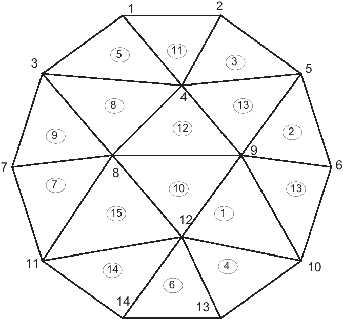
In the Fig. 95, we have the following.
\(n_v=14, n_t=16, n_s=10\)
\(q^1=(-0.309016994375, 0.951056516295)\)
\(\dots\)
\(q^{14}=(-0.309016994375, -0.951056516295)\)
The vertices of \(T_1\) are \(q^9, q^{12},\, q^{10}\).
\(\dots\)
The vertices of \(T_{16}\) are \(q^9, q^{10}, q^{6}\).
The edge of the 1st side \(L_1\) are \(q^6, q^5\).
\(\dots\)
The edge of the 10th side \(L_{10}\) are \(q^{10}, q^6\).
In FreeFEM there are many mesh file formats available for communication with other tools such as emc2, modulef, … (see Mesh format chapter ).
The extension of a file implies its format. More details can be found on the file format .msh in the article by F. Hecht “bamg : a bidimensional anisotropic mesh generator” [HECHT1998_2].
A mesh file can be read into FreeFEM except that the names of the borders are lost and only their reference numbers are kept.
So these borders have to be referenced by the number which corresponds to their order of appearance in the program, unless this number is overwritten by the keyword label. Here are some examples:
 1// Parameters
 2int n = 10;
 3
 4// Mesh
 5border floor(t=0, 1){x=t; y=0; label=1;};
 6border right(t=0, 1){x=1; y=t; label=5;};
 7border ceiling(t=1, 0){x=t; y=1; label=5;};
 8border left(t=1, 0){x=0; y=t; label=5;};
 9
10mesh th = buildmesh(floor(n) + right(n) + ceiling(n) + left(n));
11
12//save mesh in different formats
13savemesh(th, "toto.am_fmt"); // format "formated Marrocco"
14savemesh(th, "toto.Th"); // format database db mesh "bamg"
15savemesh(th, "toto.msh"); // format freefem
16savemesh(th, "toto.nopo"); // modulef format
17
18// Fespace
19fespace femp1(th, P1);
20femp1 f = sin(x)*cos(y);
21femp1 g;
22
23//save the fespace function in a file
24{
25  ofstream file("f.txt");
26  file << f[] << endl;
27} //the file is automatically closed at the end of the block
28//read a file and put it in a fespace function
29{
30  ifstream file("f.txt");
31  file >> g[] ;
32}//the file is equally automatically closed
33
34// Plot
35plot(g);
36
37// Mesh 2
38//read the mesh for freefem format saved mesh
39mesh th2 = readmesh("toto.msh");
40
41// Fespace 2
42fespace Vh2(th2, P1);
43Vh2 u, v;
44
45// Problem
46//solve:
47//  $u + \Delta u = g$ in $\Omega $
48//  $u=0$ on $\Gamma_1$
49//  $\frac{\partial u }{\partial n} = g$ on $\Gamma_2$
50solve Problem(u, v)
51  = int2d(th2)(
52      u*v
53    - dx(u)*dx(v)
54    - dy(u)*dy(v)
55  )
56  + int2d(th2)(
57    - g*v
58  )
59  + int1d(th2, 5)(
60      g*v
61  )
62  + on(1, u=0)
63  ;
64
65// Plot
66plot(th2, u);
Input/output for a mesh
the command readmesh
- The function
readmeshallows to build ameshfrom a data file 1mesh Th=readmeshS("Th.mesh"); 2mesh Thff = readmesh("Thff.msh"); // FreeFEM format
the command savemesh
- The function
savemeshallows to export amesh 1savemesh(Th,"Th.mesh") 2savemesh(Thff,"Thff.msh") // FreeFEM format 3 4savemesh(th, "toto.msh"); // format freefem savemesh(th, "toto.am_fmt"); // format "formated Marrocco" 5savemesh(th, "toto.Th"); // format database db mesh "bamg" 6savemesh(th, "toto.nopo"); // modulef format 7// allows to save the 2d mesh with the 3rd space coordinate as a scalar solution for visualise 8savemesh(Th,"mm",[x,y,u]); // save surface mesh for medit, see for example minimal-surf.edp 9exec("medit mm;rm mm.bb mm.faces mm.points");
the command vtkloadS
The function vtkload allows to build a mesh from a data mesh at vtk format mesh
1load "iovtk"
2mesh Th=vtkloadS("mymesh.vtk");
the command savevtk
- The function
savevtkallows to export ameshto a data mesh at vtk format mesh 1 load "iovtk" 2 savevtk("Th.vtk",Th);
the command gmshload
- The function
gmshloadSallows to build ameshfrom a data mesh file at formatmsh (GMSH) 1load "gmsh" 2mesh Th=gmshload("mymesh.msh");
the command savegmsh
- The function
savegmshallows to export ameshto a data mesh msh (GMSH) 1 load "gmsh" 2savegmsh(Th, "Th");
3d case
format of mesh data
In three dimensions, the file mesh format supported for input and output files by FreeFEM are the extension .msh and .mesh. These formats are described in the Mesh Format section.
Extension file .msh The structure of the files with extension .msh in 3D is given by:
In this structure, \(n_v\) denotes the number of vertices, \(n_{tet}\) the number of tetrahedra and \(n_{tri}\) the number of triangles.
For each vertex \(q^i,\, i=1,\cdots,n_v\), we denote by \((q^i_x,q^i_y,q^i_z)\) the \(x\)-coordinate, the \(y\)-coordinate and the \(z\)-coordinate.
Each tetrahedra \(T_k, k=1,\cdots,n_{tet}\) has four vertices \(q^{k_1},\, q^{k_2},\,q^{k_3}, \,q^{k_4}\).
The boundary consists of a union of triangles. Each triangle \(tri_j, j=1,\cdots,n_{tri}\) has three vertices \(q^{j_1},\, q^{j_2},\,q^{j_3}\).
extension file .mesh The data structure for a three dimensional mesh is composed of the data structure presented in Mesh Format section and a data structure for the tetrahedra. The tetrahedra of a three dimensional mesh are referred using the following field:
 1Tetrahedra
 2NbTetrahedra
 3Vertex1 Vertex2 Vertex3 Vertex4 Label
 4...
 5Vertex1 Vertex2 Vertex3 Vertex4 Label
 6Triangles
 7NbTriangles
 8Vertex1 Vertex2 Vertex3 Label
 9...
10Vertex1 Vertex2 Vertex3 Label
This field is express with the notation of Mesh Format section.
Input/output for a mesh3
the command readmesh3
- The function
readmesh3allows to build amesh3from a data file 1mesh3 Th3=readmesh3("Th3.mesh"); 2mesh3 Th3ff = readmesh3("Th3ff.msh"); // FreeFEM format
the command savemesh
- The function
savemeshallows to export amesh3 1savemesh(Th3,"Th3.mesh") 2savemesh(Th3ff,"Th3ff.msh") // FreeFEM format
the command vtkload3
The function vtkload3 allows to build a mesh3 from a data mesh at vtk format mesh
1load "iovtk"
2mesh3 Th3=vtkloadS("mymesh.vtk");
the command savevtk
- The function
savevtkallows to export amesh3to a data mesh at vtk format mesh 1 load "iovtk" 2 savevtk("Th3.vtk",Th3);
the command gmshload3
- The function
gmshload3allows to build amesh3from a data mesh file at formatmsh (GMSH) 1load "gmsh" 2mesh3 Th3=gmshload3("mymesh.msh");
the command savegmsh
- The function
savegmshallows to export amesh3to a data mesh msh (GMSH) 1 load "gmsh" 2savegmsh(Th3, "Th3");
Surface 3d case
format of mesh data
Like 2d and 3d, the input and output format files supported by FreeFEM are the extension .msh and .mesh. These formats are described in the Mesh Format section.
Extension file .msh The structure of the files with extension .msh in surface 3D is given by:
In this structure, \(n_v\) denotes the number of vertices, \(n_{tet}\) the number of tetrahedra and \(n_{tri}\) the number of triangles.
For each vertex \(q^i,\, i=1,\cdots,n_v\), we denote by \((q^i_x,q^i_y,q^i_z)\) the \(x\)-coordinate, the \(y\)-coordinate and the \(z\)-coordinate.
Each tetrahedra \(T_k, k=1,\cdots,n_{tet}\) has four vertices \(q^{k_1},\, q^{k_2},\,q^{k_3}, \,q^{k_4}\).
The boundary consists of a union of triangles. Each triangle \(be_j, j=1,\cdots,n_{tri}\) has three vertices \(q^{j_1},\, q^{j_2},\,q^{j_3}\).
extension file .mesh The data structure for a three dimensional mesh is composed of the data structure presented in Mesh Format section and a data structure for the tetrahedra. The tetrahedra of a three dimensional mesh are referred using the following field:
 1MeshVersionFormatted 2
 2Dimension 3
 3
 4Vertices
 5NbVertices
 6(v0)x (v0)y (v0)z
 7...
 8(vn)x (vn)y (vn)z
 9
10Triangles
11NbTriangles
12Vertex1 Vertex2 Vertex3 Label
13...
14Vertex1 Vertex2 Vertex3 Label
15
16Edges
17NbEdges
18Vertex1 Vertex2 Label
19...
20Vertex1 Vertex2 Label
21
22End
This field is express with the notation of Mesh Format section.
Input/output for a meshS
the command readmesh3
- The function
readmeshSallows to build ameshSfrom a data file 1meshS ThS=readmeshS("ThS.mesh"); 2meshS Th3ff = readmeshS("ThSff.msh"); // FreeFEM format
the command savemesh
- The function
savemeshallows to export ameshS 1savemesh(ThS,"ThS.mesh") 2savemesh(ThSff,"ThSff.msh") // FreeFEM format
the command vtkloadS
The function vtkloadS allows to build a meshS from a data mesh at vtk format mesh
1load "iovtk"
2meshS ThS=vtkloadS("mymesh.vtk");
the command savevtk
- The function
savevtkallows to export ameshSto a data mesh at vtk format mesh 1 load "iovtk" 2 savevtk("ThS.vtk",ThS);
the command gmshloadS
- The function
gmshloadSallows to build ameshSfrom a data mesh file at formatmsh (GMSH) 1load "gmsh" 2meshS ThS=gmshloadS("mymesh.msh");
the command savegmsh
- The function
savegmshallows to export ameshSto a data mesh msh (GMSH) 1 load "gmsh" 2savegmsh(ThS, "ThS");
Medit
The keyword medit allows to display a mesh alone or a mesh and one or several functions defined on the mesh using the Pascal Frey’s freeware medit.
medit opens its own window and uses OpenGL extensively.
Naturally to use this command medit must be installed.
A vizualisation with medit of scalar solutions \(f1\) and \(f2\) continuous, piecewise linear and known at the vertices of the mesh Th is obtained using:
1medit("sol1 sol2", Th, f1, f2, order=1);
The first plot named sol1 display f1.
The second plot names sol2 display f2.
The arguments of the function medit are the name of the differents scenes (separated by a space) of medit, a mesh and solutions.
Each solution is associated with one scene.
The scalar, vector and symmetric tensor solutions are specified in the format described in the section dealing with the keyword savesol.
The parameters of this command line are :
order=0 if the solution is given at the center of gravity of elements.1 is the solution is given at the vertices of elements.
meditff=set the name of execute command of medit.By default, this string is medit.
save=set the name of a file.solor.solbto save solutions.
This command line allows also to represent two differents meshes and solutions on them in the same windows. The nature of solutions must be the same. Hence, we can vizualize in the same window the different domains in a domain decomposition method for instance. A vizualisation with medit of scalar solutions \(h1\) and \(h2\) at vertices of the mesh Th1 and Th2 respectively are obtained using:
1medit("sol2domain", Th1, h1, Th2, h2, order=1);
Tip
Medit
 1load "medit"
 2
 3// Initial Problem:
 4// Resolution of the following EDP:
 5// -Delta u_s = f on \Omega = { (x,y) | 1 <= sqrt(x^2+y^2) <= 2 }
 6// -Delta u_1 = f1 on \Omega_1 = { (x,y) | 0.5 <= sqrt(x^2+y^2) <= 1. }
 7// u = 1 on Gamma
 8// Null Neumman condition on Gamma_1 and on Gamma_2
 9// We find the solution u by solving two EDP defined on domain Omega and Omega_1
10// This solution is visualize with medit
11
12verbosity=3;
13
14// Mesh
15border Gamma(t=0, 2*pi){x=cos(t); y=sin(t); label=1;};
16border Gamma1(t=0, 2*pi){x=2*cos(t); y=2*sin(t); label=2;};
17border Gamma2(t=0, 2*pi){x=0.5*cos(t); y=0.5*sin(t); label=3;};
18
19mesh Th = buildmesh(Gamma1(40) + Gamma(-40)); //Omega
20mesh Th1 = buildmesh(Gamma(40) + Gamma2(-40)); //Omega_1
21
22// Fespace
23fespace Vh(Th, P2);
24func f = sqrt(x*x + y*y);
25Vh us, v;
26
27fespace Vh1(Th1, P2);
28func f1 = 10*sqrt(x*x+y*y);
29Vh1 u1, v1;
30
31// Macro
32macro Grad2(us) [dx(us), dy(us)] // EOM
33
34// Problem
35problem Lap2dOmega (us, v, init=false)
36    = int2d(Th)(
37        Grad2(v)' * Grad2(us)
38    )
39    - int2d(Th)(
40        f*v
41    )
42    +on(1, us=1)
43    ;
44
45problem Lap2dOmega1 (u1, v1, init=false)
46    = int2d(Th1)(
47        Grad2(v1)' * Grad2(u1)
48    )
49    - int2d(Th1)(
50        f1*v1
51    )
52    + on(1, u1=1)
53    ;
54
55// Solve
56Lap2dOmega;
57Lap2dOmega1;
58
59// Plot with medit
60medit("solution", Th, us, Th1, u1, order=1, save="testsavemedit.solb");
Mshmet
Mshmet is a software developed by P. Frey that allows to compute an anisotropic metric based on solutions (i.e. Hessian-based).
This software can return also an isotropic metric.
Moreover, mshmet can also construct a metric suitable for levelset interface capturing.
The solution can be defined on 2D or 3D structured/unstructured meshes.
For example, the solution can be an error estimate of a FE solution.
Solutions for mshmet are given as an argument.
The solution can be a func, a vector func, a symmetric tensor, a fespace function, a fespace vector function and a fespace symmetric tensor.
The symmetric tensor argument is defined as this type of data for datasol argument.
This software accepts more than one solution.
For example, the metric \(M\) computed with mshmet for the solution \(u\) defined on the mesh \(Th\) is obtained by writing:
1fespace Vh(Th, P1);
2Vh u; //a scalar fespace function
3real[int] M = mshmet(Th, u);
The parameters of the keyword mshmet are :
normalization =(b) do a normalization of all solution in \([0,1]\).aniso =(b) build anisotropic metric if 1 (default 0: isotropic)levelset =(b) build metric for levelset method (default:false)verbosity =(l) level of verbositynbregul =(l) number of regularization’s iteration of solutions given (default 0).hmin =(d)hmax =(d)err =(d) level of error.width =(d) the widthmetric =a vector of double.This vector contains an initial metric given to
mshmet. The structure of the metric vector is described in the next paragraph.
loptions =a vector of integer of size 7.This vector contains the integer parameters of
mshmet(for expert only).loptions(0): normalization (default 1).
- loptions(1): isotropic parameters (default 0).
1 for isotropic metric results otherwise 0.
- loptions(2): level set parameters (default 0).
1 for building level set metric otherwise 0.
- loptions(3): debug parameters (default 0).
1 for turning on debug mode otherwise 0.
loptions(4): level of verbosity (default 10).
loptions(5): number of regularization’s iteration of solutions given (default 0).
- loptions(6): previously metric parameter (default 0).
1 for using previous metric otherwise 0.
doptions=a vector of double of size 4.This vector contains the real parameters of
mshmet(for expert only).doptions(0): hmin : min size parameters (default 0.01).
doptions(1): hmax : max size parameters (default 1.0).
doptions(2): eps : tolerance parameters (default 0.01).
doptions(2): width : relative width for Level Set (\(0<w<1\)) (default 0.05).
The result of the keyword mshmet is a real[int] which contains the metric computed by mshmet at the different vertices \(V_{i}\) of the mesh.
With \(nv\) is the number of vertices, the structure of this vector is:
for a isotropic metric \(m\).
For a symmetric tensor metric \(h=\left(\begin{array}{ccc} m_{1 1} & m_{1 2} & m_{1 3}\\ m_{2 1} & m_{2 2} & m_{2 3} \\ m_{3 1} & m_{3 2} & m_{3 3} \end{array}\right)\) , the parameters metric is:
where \(H(V_{i})\) is the vector of size 6 defined by \([m11,m21,m22,m31,m32,m33]\)
Tip
mshmet
 1load "mshmet"
 2load "medit"
 3load "msh3"
 4
 5// Parameters
 6real error = 0.01;
 7func zmin = 0;
 8func zmax = 1;
 9int MaxLayer = 10;
10
11// Mesh
12border a(t=0, 1.0){x=t; y=0; label=1;};
13border b(t=0, 0.5){x=1; y=t; label=2;};
14border c(t=0, 0.5){x=1-t; y=0.5; label=3;};
15border d(t=0.5, 1){x=0.5; y=t; label=4;};
16border e(t=0.5, 1){x=1-t; y=1; label=5;};
17border f(t=0.0, 1){x=0; y=1-t; label=6;};
18mesh Th = buildmesh(a(6) + b(4) + c(4) + d(4) + e(4) + f(6));
19mesh3 Th3 = buildlayers(Th, MaxLayer, zbound=[zmin, zmax]);
20
21// Fespace
22fespace Vh3(Th3, P2);
23Vh3 u3, v3;
24
25fespace Vh3P1(Th3, P1);
26Vh3P1 usol;
27
28// Problem
29problem Problem2(u3, v3, solver=sparsesolver)
30    = int3d(Th3)(
31        u3*v3*1.0e-10
32        + dx(u3)*dx(v3)
33        + dy(u3)*dy(v3)
34        + dz(u3)*dz(v3)
35    )
36    - int3d(Th3)(
37        v3
38    )
39    +on(0, 1, 2, 3, 4, 5, 6, u3=0)
40    ;
41
42// Solve
43Problem2;
44cout << u3[].min << " " << u3[].max << endl;
45
46medit("Sol", Th3, u3);
47
48real[int] bb = mshmet(Th3,u3);
49cout << "Metric:" << bb << endl;
50for (int ii = 0; ii < Th3.nv; ii++)
51    usol[][ii] = bb[ii];
52
53medit("Metric", Th3, usol);
FreeYams
FreeYams is a surface mesh adaptation software which is developed by P. Frey. This software is a new version of yams. The adapted surface mesh is constructed with a geometric metric tensor field. This field is based on the intrinsic properties of the discrete surface.
Also, this software allows to construct a simplification of a mesh. This decimation is based on the Hausdorff distance between the initial and the current triangulation. Compared to the software yams, FreeYams can be used also to produce anisotropic triangulations adapted to levelset simulations. A technical report on freeYams documentation is available here.
To call FreeYams in FreeFEM, we used the keyword freeyams.
The arguments of this function are the initial mesh and/or metric.
The metric with freeyams are a func, a fespace function, a symmetric tensor function, a symmetric tensor fespace function or a vector of double (real[int]).
If the metric is a vector of double, this data must be given in metric parameter.
Otherwise, the metric is given in the argument.
For example, the adapted mesh of Thinit defined by the metric \(u\) defined as fespace function is obtained by writing:
1fespace Vh(Thinit, P1);
2Vh u;
3mesh3 Th = freeyams(Thinit, u);
The symmetric tensor argument for freeyams keyword is defined as this type of data for datasol argument.
aniso=(b) aniso or iso metric (default 0, iso)mem=(l) memory of for freeyams in Mb (default -1, freeyams choose)hmin=(d)hmax=(d)gradation=(d)option=(l)0 : mesh optimization (smoothing+swapping)
1 : decimation+enrichment adaptated to a metric map. (default)
-1 : decimation adaptated to a metric map.
2 : decimation+enrichment with a Hausdorff-like method
-2 : decimation with a Hausdorff-like method
4 : split triangles recursively.
9 : No-Shrinkage Vertex Smoothing
ridgeangle=(d)absolute=(b)verbosity=(i)metric=vector expression.This parameters contains the metric at the different vertices on the initial mesh. With \(nv\) is the number of vertices, this vector is:
\[M_{iso}= ( m(V_0), m(V_1), \ldots, m(V_{nv}) )^t\]for a scalar metric \(m\). For a symmetric tensor metric \(h=\left(\begin{array}{ccc} m_{1 1} & m_{1 2} & m_{1 3}\\ m_{2 1} & m_{2 2} & m_{2 3} \\ m_{3 1} & m_{3 2} & m_{3 3} \end{array}\right)\), the parameters
metricis:\[M_{aniso}= ( H(V_{0}), \ldots, H(V_{nv}) )^t\]where \(H(V_{i})\) is the vector of size 6 defined by \([m11,m21,m22,m31,m32,m33]\)
loptions=a vector of integer of size 13.This vectors contains the integer options of FreeYams. (just for the expert)
- loptions(0): anisotropic parameter (default 0).
If you give an anisotropic metric 1 otherwise 0.
- loptions(1): Finite Element correction parameter (default 0).
1 for no Finite Element correction otherwise 0.
- loptions(2): Split multiple connected points parameter (default 1).
1 for splitting multiple connected points otherwise 0.
loptions(3): maximum value of memory size in Mbytes (default -1: the size is given by freeyams).
- loptions(4): set the value of the connected component which we want to obtain.
(Remark: freeyams give an automatic value at each connected component).
loptions(5): level of verbosity
- loptions(6): Create point on straight edge (no mapping) parameter (default 0).
1 for creating point on straight edge otherwise 0.
- loptions(7): validity check during smoothing parameter.
This parameter is only used with No-Shrinkage Vertex Smoothing optimization (optimization option parameter 9). 1 for No validity checking during smoothing otherwise 0.
loptions(8): number of desired’s vertices (default -1).
loptions(9): number of iteration of optimizations (default 30).
- loptions(10): no detection parameter (default 0).
1 for detecting the ridge on the mesh otherwise 0. The ridge definition is given in the parameter doptions(12).
- loptions(11): no vertex smoothing parameter (default 0).
1 for smoothing the vertices otherwise 0.
loptions(12): Optimization level parameter (default 0).
0 : mesh optimization (smoothing+swapping)
1 : decimation+enrichment adaptated to a metric map.
-1: decimation adaptated to a metric map.
2 : decimation+enrichment with a Hausdorff-like method
-2: decimation with a Hausdorff-like method
4 : split triangles recursively.
9 : No-Shrinkage Vertex Smoothing
doptions=a vector of double of size 11.This vectors contains the real options of freeyams.
doptions(0): Set the geometric approximation (Tangent plane deviation) (default 0.01).
doptions(1): Set the lamda parameter (default -1).
doptions(2): Set the mu parmeter (default -1).
doptions(3): Set the gradation value (Mesh density control) (default 1.3).
doptions(4): Set the minimal size(hmin) (default -2.0: the size is automatically computed).
doptions(5): Set the maximal size(hmax) (default -2.0: the size is automatically computed).
doptions(6): Set the tolerance of the control of Chordal deviation (default -2.0).
doptions(7): Set the quality of degradation (default 0.599).
doptions(8): Set the declic parameter (default 2.0).
doptions(9): Set the angular walton limitation parameter (default 45 degree).
doptions(10): Set the angular ridge detection (default 45 degree).
Tip
freeyams
 1load "msh3"
 2load "medit"
 3load "freeyams"
 4
 5// Parameters
 6int nn = 20;
 7real zmin = 0;
 8real zmax = 1;
 9
10// Mesh
11mesh Th2 = square(nn, nn);
12int[int] rup = [0, 2], rdown = [0, 1];
13int[int] rmid = [1, 1, 2, 1, 3, 1, 4, 1];
14mesh3 Th = buildlayers(Th2, nn, zbound=[zmin, zmax], reffacemid=rmid, reffaceup=rup, reffacelow=rdown);
15mesh3 Th3 = freeyams(Th);
16
17medit("SurfaceMesh", Th3);
mmg3d
Todo
mmg3d-v4.0
Mmg3d is a 3D remeshing software developed by C. Dobrzynski and P. Frey.
This software allows to remesh an initial mesh made of tetrahedra. This initial mesh is adapted to a geometric metric tensor field or to a displacement vector (moving rigid body). The metric can be obtained with mshmet.
Note
If no metric is given, an isotropic metric is computed by analyzing the size of the edges in the initial mesh.
If a displacement is given, the vertices of the surface triangles are moved without verifying the geometrical structure of the new surface mesh.
The parameters of mmg3d are :
options=vector expression.This vector contains the option parameters of
mmg3d. It is a vector of 6 values, with the following meaning:
Optimization parameters : (default 1)
0 : mesh optimization.
1 : adaptation with metric (deletion and insertion vertices) and optimization.
-1 : adaptation with metric (deletion and insertion vertices) without optimization.
4 : split tetrahedra (be careful modify the surface).
9 : moving mesh with optimization.
-9 : moving mesh without optimization.
Debug mode : (default 0)
1 : turn on debug mode.
0 : otherwise.
Specify the size of bucket per dimension (default 64)
Swapping mode : (default 0)
1 : no edge or face flipping.
0 : otherwise.
Insert points mode : (default 0)
1 : no edge splitting or collapsing and no insert points.
0 : otherwise.
Verbosity level (default 3)
memory=integer expression.Set the maximum memory size of new mesh in Mbytes. By default the number of maximum vertices, tetrahedra and triangles are respectively 500 000, 3000 000, 100000 which represent approximately a memory of 100 Mo.
metric=vector expression.This vector contains the metric given at
mmg3d. It is a vector of size \(nv\) or 6 \(nv\) respectively for an isotropic and anisotropic metric where \(nv\) is the number of vertices in the initial mesh. The structure ofmetricvector is described in the mshmet.
displacement=\([\Phi1, \Phi2, \Phi3]\) set the displacement vector of the initial mesh \(\mathbf{\Phi(x,y)} = [\Phi1(x,y), \Phi2(x,y), \Phi3(x,y)]\).displVect=sets the vector displacement in a vector expression.This vector contains the displacement at each point of the initial mesh. It is a vector of size 3 \(nv\).
Tip
mmg3d
 1load "msh3"
 2load "medit"
 3load "mmg3d"
 4include "Cube.idp"
 5
 6// Parameters
 7int n = 6;
 8int[int] Nxyz = [12, 12, 12];
 9real [int, int] Bxyz = [[0., 1.], [0., 1.], [0., 1.]];
10int [int, int] Lxyz = [[1, 1], [2, 2], [2, 2]];
11
12// Mesh
13mesh3 Th = Cube(Nxyz, Bxyz, Lxyz);
14
15real[int] isometric(Th.nv);
16for (int ii = 0; ii < Th.nv; ii++)
17    isometric[ii] = 0.17;
18
19mesh3 Th3 = mmg3d(Th, memory=100, metric=isometric);
20
21// Plot
22medit("Initial", Th);
23medit("Isometric", Th3);
Tip
Falling spheres
 1load "msh3"
 2load "TetGen"
 3load "medit"
 4load "mmg3d"
 5include "MeshSurface.idp"
 6
 7// Parameters
 8real hs = 0.8;
 9int[int] N = [4/hs, 8/hs, 11.5/hs];
10real [int, int] B = [[-2, 2], [-2, 6], [-10, 1.5]];
11int [int, int] L = [[311, 311], [311, 311], [311, 311]];
12
13int[int] opt = [9, 0, 64, 0, 0, 3];
14real[int] vit=[0, 0, -0.3];
15func zero = 0.;
16func dep = vit[2];
17
18// Meshes
19meshS ThH = SurfaceHex(N, B, L, 1);
20meshS ThSg = Sphere(1, hs, 300, -1);
21meshS ThSd = Sphere(1, hs, 310, -1);
22ThSd = movemesh(ThSd, [x, 4+y, z]);
23meshS ThHS = ThH + ThSg + ThSd;
24medit("ThHS", ThHS);
25
26real voltet = (hs^3)/6.;
27real[int] domain = [0, 0, -4, 1, voltet];
28real [int] holes = [0, 0, 0, 0, 4, 0];
29mesh3 Th = tetg(ThHS, switch="pqaAAYYQ", nbofregions=1, regionlist=domaine, nbofholes=2, holelist=holes);
30medit("Box-With-two-Ball", Th);
31
32// Fespace
33fespace Vh(Th, P1);
34Vh uh,vh;
35
36// Macro
37macro Grad(u) [dx(u),dy(u),dz(u)]
38
39// Problem
40problem Lap (uh, vh, solver=CG)
41    = int3d(Th)(
42        Grad(uh)' * Grad(vh)
43    )
44    + on(310, 300, uh=dep)
45    + on(311, uh=0.)
46    ;
47
48// Falling loop
49for(int it = 0; it < 29; it++){
50    cout << " ITERATION " << it << endl;
51
52    // Solve
53    Lap;
54
55    // Plot
56    plot(Th, uh);
57
58    // Sphere falling
59    Th = mmg3d(Th, options=opt, displacement=[zero, zero, uh], memory=1000);
60}
A first 3d isotrope mesh adaptation process
Tip
Adaptation 3D
 1load "msh3"
 2load "TetGen"
 3load "mshmet"
 4load "medit"
 5
 6// Parameters
 7int nn = 6;
 8int[int] l1111 = [1, 1, 1, 1]; //labels
 9int[int] l01 = [0, 1];
10int[int] l11 = [1, 1];
11
12real errm = 1e-2; //level of error
13
14// Mesh
15mesh3 Th3 = buildlayers(square(nn, nn, region=0, label=l1111),
16nn, zbound=[0, 1], labelmid=l11, labelup=l01, labeldown=l01);
17
18Th3 = trunc(Th3, (x<0.5) | (y < 0.5) | (z < 0.5), label=1); //remove the ]0.5,1[^3 cube
19
20// Fespace
21fespace Vh(Th3, P1);
22Vh u, v, usol, h;
23
24// Macro
25macro Grad(u) [dx(u), dy(u), dz(u)] // EOM
26
27// Problem
28problem Poisson (u, v, solver=CG)
29    = int3d(Th3)(
30        Grad(u)' * Grad(v)
31    )
32    - int3d(Th3)(
33        1*v
34    )
35    + on(1, u=0)
36    ;
37
38// Loop
39for (int ii = 0; ii < 5; ii++){
40    // Solve
41    Poisson;
42    cout << "u min, max = " << u[].min << " "<< u[].max << endl;
43
44    h=0.; //for resizing h[] because the mesh change
45    h[] = mshmet(Th3, u, normalization=1, aniso=0, nbregul=1, hmin=1e-3, hmax=0.3, err=errm);
46    cout << "h min, max = " << h[].min << " "<< h[].max << " " << h[].n << " " << Th3.nv << endl;
47    plot(u, wait=true);
48
49    errm *= 0.8; //change the level of error
50    cout << "Th3 " << Th3.nv < " " << Th3.nt << endl;
51    Th3 = tetgreconstruction(Th3, switch="raAQ", sizeofvolume=h*h*h/6.); //rebuild mesh
52    medit("U-adap-iso-"+ii, Th3, u, wait=true);
53}
Build a 2d mesh from an isoline
The idea is to get the discretization of an isoline of fluid meshes, this tool can be useful to construct meshes from image. First, we give an example of the isovalue meshes \(0.2\) of analytical function \(\sqrt{(x-1/2)^2 +(y-1/2)^2}\), on unit square.
 1load "isoline"
 2
 3real[int,int] xy(3, 1); //to store the isoline points
 4int[int] be(1); //to store the begin, end couple of lines
 5{
 6    mesh Th = square(10, 10);
 7    fespace Vh(Th, P1);
 8    Vh u = sqrt(square(x-0.5) + square(y-0.5));
 9    real iso = 0.2 ;
10    real[int] viso = [iso];
11    plot(u, viso=viso,Th);//to see the iso line
12
13    int nbc = isoline(Th, u, xy, close=1, iso=iso, beginend=be, smoothing=0.1);
The isoline parameters are Th the mesh, the expression \(u\), the bidimentionnal array xy to store the list coordinate of the points.
The list of named parameter are :
iso=value of the isoline to compute (0 is the default value)close=close the isoline with the border (defaulttrue), we add the part of the mesh border such the value is less than the isovaluesmoothing=number of smoothing process is the \({l} ^{r} {s}\) where \(l\) is the length of the current line component, \(r\) the ratio, \(s\) is smoothing value. The smoothing default value is 0.ratio=the ratio (1 by default).eps=relative \(\varepsilon\) (default 1e-10)beginend=array to get begin, end couple of each of sub line (resize automatically)file=to save the data curve in data file for gnuplot
In the array xy you get the list of vertices of the isoline, each connex line go from \(i= i_0^c ,\dots, i_1^c-1\) with \(i_0^c =be(2*c)\) \(i_1^c =be(2*c+1)\), and where \(x_i= xy(0,i), y_i=yx( 1,i), l_i=xy(2,i)\).
Here \(l_i\) is the length of the line (the origin of the line is point \(i_0^c\)).
The sense of the isoline is such that the upper part is at the left size of the isoline. So here : the minimum is a point \(0.5,05\) so the curve 1 turn in the clockwise sense, the order of each component are sort such that the number of point by component is decreasing.
 1      cout << "Number of the line component = " << nbc << endl;
 2      cout << "Number of points = " << xy.m << endl;
 3      cout << "be = " << be << endl;
 4
 5      // shows the lines component
 6      for (int c = 0; c < nbc; ++c){
 7         int i0 = be[2*c], i1 = be[2*c+1]-1;
 8         cout << "Curve " << c << endl;
 9         for(int i = i0; i <= i1; ++i)
10            cout << "x= " << xy(0,i) << " y= " << xy(1,i) << " s= " << xy(2, i) << endl;
11         plot([xy(0, i0:i1), xy(1, i0:i1)], wait=true, viso=viso, cmm=" curve "+c);
12   }
13}
14
15cout << "length of last curve = " << xy(2, xy.m-1) << endl;
We also have a new function to easily parametrize a discrete curve defined by the couple \(be, xy\).
 1border Curve0(t=0, 1){
 2    int c=0; //component 0
 3    int i0=be[2*c], i1=be[2*c+1]-1;
 4    P=Curve(xy, i0, i1, t); //Curve 0
 5    label=1;
 6}
 7
 8border Curve1(t=0, 1){
 9    int c=1; //component 1
10    int i0=be[2*c], i1=be[2*c+1]-1;
11    P=Curve(xy, i0, i1, t); //Curve 1
12    label=1;
13}
14
15plot(Curve1(100)); //show curve
16mesh Th = buildmesh(Curve1(-100));
17plot(Th, wait=true);
Secondly, we use this idea to build meshes from an image, we use the plugins ppm2rnm to read pgm a gray scale image and then we extract the gray contour at level 0.25.
Tip
Leman lake
 1load "ppm2rnm"
 2load "isoline"
 3
 4// Parameters
 5string leman = "LemanLake.pgm";
 6real AreaLac = 580.03; //in km^2
 7real hsize = 5;
 8real[int, int] Curves(3, 1);
 9int[int] be(1);
10int nc; //nb of curve
11{
12    real[int, int] ff1(leman); //read image
13    //and set it in a rect. array
14    int nx = ff1.n, ny = ff1.m;
15    //build a Cartesian mesh such that the origin is in the right place.
16    mesh Th = square(nx-1, ny-1, [(nx-1)*(x), (ny-1)*(1-y)]);
17    //warning the numbering of the vertices (x,y) is
18    //given by $i = x/nx + nx* y/ny $
19    fespace Vh(Th, P1);
20    Vh f1;
21    f1[] = ff1; //transform array in finite element functions.
22    nc = isoline(Th, f1, iso=0.25, close=1, Curves, beginend=be, smoothing=.1, ratio=0.5);
23}
24
25//The longest isoline: the lake
26int ic0 = be(0), ic1 = be(1)-1;
27plot([Curves(0, ic0:ic1), Curves(1, ic0:ic1)], wait=true);
28
29int NC = Curves(2, ic1)/hsize;
30real xl = Curves(0, ic0:ic1).max - 5;
31real yl = Curves(1, ic0:ic1).min + 5;
32border G(t=0, 1){P=Curve(Curves, ic0, ic1, t); label=1+(x>xl)*2+(y<yl);}
33plot(G(-NC), wait=true);
34
35mesh Th = buildmesh(G(-NC));
36plot(Th, wait=true);
37
38real scale = sqrt(AreaLac/Th.area);
39Th = movemesh(Th, [x*scale, y*scale]);
40cout << "Th.area = " << Th.area << " Km^2 " << " == " << AreaLac << " Km^2 " << endl;
41plot(Th, wait=true, ps="leman.eps");