Membrane

Summary : Here we shall learn how to solve a Dirichlet and/or mixed Dirichlet Neumann problem for the Laplace operator with application to the equilibrium of a membrane under load. We shall also check the accuracy of the method and interface with other graphics packages

An elastic membrane \(\Omega\) is attached to a planar rigid support \(\Gamma\), and a force \(f(x) dx\) is exerted on each surface element \(\text{d}{x}=\text{d}{x}_1 \text{d}{x}_2\). The vertical membrane displacement, \(\varphi(x)\), is obtained by solving Laplace’s equation:

\[-\Delta \varphi =f ~\hbox{in}~ \Omega\]

As the membrane is fixed to its planar support, one has:

\[\varphi |_{\Gamma }=0\]

If the support wasn’t planar but had an elevation \(z(x_1,x_2)\) then the boundary conditions would be of non-homogeneous Dirichlet type.

\[\varphi|_{\Gamma}=z\]

If a part \(\Gamma_2\) of the membrane border \(\Gamma\) is not fixed to the support but is left hanging, then due to the membrane’s rigidity the angle with the normal vector \(\boldsymbol{n}\) is zero; thus the boundary conditions are:

\[\varphi|_{\Gamma_1}=z,~~~~\frac{\partial\varphi}{\partial\boldsymbol{n}}|_{\Gamma_2}=0\]

where \(\Gamma_1=\Gamma-\Gamma_2\); recall that \(\frac{\partial\varphi}{\partial\boldsymbol{n}}=\nabla\varphi\cdot \boldsymbol{n}\) Let us recall also that the Laplace operator \(\Delta\) is defined by:

\[\Delta \varphi = {\partial ^{2}\varphi \over \partial x^{2}_{1} } + {\partial ^{2}\varphi \over \partial x_{2}^{2} }\]

Todo

Check references

With such “mixed boundary conditions” the problem has a unique solution (see Dautray-Lions (1988), Strang (1986) and Raviart-Thomas (1983)). The easiest proof is to notice that \(\varphi\) is the state of least energy, i.e.

\[E(\phi) =\min_{\varphi-z\in V} E(v) ,\quad \mbox{with} \quad E(v)=\int_\Omega(\frac12|\nabla v|^2-fv )\]

and where \(V\) is the subspace of the Sobolev space \(H^1(\Omega)\) of functions which have zero trace on \(\Gamma_1\). Recall that (\(x\in\mathbb{R}^d,~d=2\) here):

\[H^1(\Omega)=\{u\in L^2(\Omega)~:~\nabla u\in (L^2(\Omega))^d\}\]

Calculus of variation shows that the minimum must satisfy, what is known as the weak form of the PDE or its variational formulation (also known here as the theorem of virtual work)

\[\int_\Omega \nabla\varphi\cdot\nabla w = \int_\Omega f w\quad\forall w\in V\]

Next an integration by parts (Green’s formula) will show that this is equivalent to the PDE when second derivatives exist.

Warning

Unlike the previous version Freefem+ which had both weak and strong forms, FreeFEM implements only weak formulations. It is not possible to go further in using this software if you don’t know the weak form (i.e. variational formulation) of your problem: either you read a book, or ask help form a colleague or drop the matter. Now if you want to solve a system of PDE like \(A(u,v)=0,~ B(u,v)=0\) don’t close this manual, because in weak form it is

\[\int_\Omega(A(u,v)w_1+B(u,v)w_2)=0~~\forall w_1,w_2...\]

Example

Let an ellipse have the length of the semimajor axis \(a=2\), and unitary the semiminor axis. Let the surface force be \(f=1\). Programming this case with FreeFEM gives:

// Parameters
real theta = 4.*pi/3.;
real a = 2.; //The length of the semimajor axis
real b = 1.; //The length of the semiminor axis
func z = x;

// Mesh
border Gamma1(t=0., theta){x=a*cos(t); y=b*sin(t);}
border Gamma2(t=theta, 2.*pi){x=a*cos(t); y=b*sin(t);}
mesh Th = buildmesh(Gamma1(100) + Gamma2(50));

// Fespace
fespace Vh(Th, P2); //P2 conforming triangular FEM
Vh phi, w, f=1;

// Solve
solve Laplace(phi, w)
    = int2d(Th)(
          dx(phi)*dx(w)
        + dy(phi)*dy(w)
    )
    - int2d(Th)(
          f*w
    )
    + on(Gamma1, phi=z)
    ;

// Plot
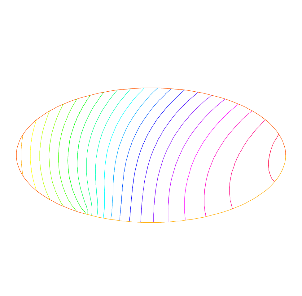
plot(phi, wait=true, ps="membrane.eps"); //Plot phi
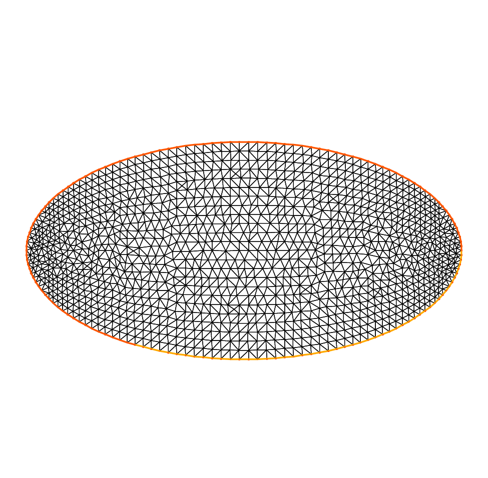
plot(Th, wait=true, ps="membraneTh.eps"); //Plot Th

// Save mesh
savemesh(Th,"Th.msh");

A triangulation is built by the keyword buildmesh. This keyword calls a triangulation subroutine based on the Delaunay test, which first triangulates with only the boundary points, then adds internal points by subdividing the edges. How fine the triangulation becomes is controlled by the size of the closest boundary edges.

The PDE is then discretized using the triangular second order finite element method on the triangulation; as was briefly indicated in the previous chapter, a linear system is derived from the discrete formulation whose size is the number of vertices plus the number of mid-edges in the triangulation.

The system is solved by a multi-frontal Gauss LU factorization implemented in the package UMFPACK.

The keyword plot will display both \(\T_h\) and \(\varphi\) (remove Th if \(\varphi\) only is desired) and the qualifier fill=true replaces the default option (colored level lines) by a full color display.

plot(phi,wait=true,fill=true); //Plot phi with full color display

Results are on Fig. 5 and Fig. 6.

Membrane

Next we would like to check the results !

One simple way is to adjust the parameters so as to know the solutions. For instance on the unit circle a=1, \(\varphi_e=\sin(x^2+y^2-1)\) solves the problem when:

\[z=0, f=-4(\cos(x^2+y^2-1)-(x^2+y^2)\sin(x^2+y^2-1))\]

except that on \(\Gamma_2\) \(\partial_n\varphi=2\) instead of zero. So we will consider a non-homogeneous Neumann condition and solve:

\[\int_\Omega\nabla\varphi\cdot\nabla w = \int_\Omega f w+\int_{\Gamma_2}2w\quad\forall w\in V\]

We will do that with two triangulations, compute the \(L^2\) error:

\[\epsilon = \int_\Omega|\varphi-\varphi_e|^2\]

and print the error in both cases as well as the log of their ratio an indication of the rate of convergence.

//  Parameters
verbosity = 0; //to remove all default output
real theta = 4.*pi/3.;
real a=1.; //the length of the semimajor axis
real b=1.; //the length of the semiminor axis
func f = -4*(cos(x^2+y^2-1) - (x^2+y^2)*sin(x^2+y^2-1));
func phiexact = sin(x^2 + y^2 - 1);

// Mesh
border Gamma1(t=0., theta){x=a*cos(t); y=b*sin(t);}
border Gamma2(t=theta, 2.*pi){x=a*cos(t); y=b*sin(t);}

// Error loop
real[int] L2error(2); //an array of two values
for(int n = 0; n < 2; n++){
    // Mesh
    mesh Th = buildmesh(Gamma1(20*(n+1)) + Gamma2(10*(n+1)));

    // Fespace
    fespace Vh(Th, P2);
    Vh phi, w;

    // Solve
    solve Laplace(phi, w)
        = int2d(Th)(
              dx(phi)*dx(w)
            + dy(phi)*dy(w)
        )
        - int2d(Th)(
              f*w
        )
        - int1d(Th, Gamma2)(
              2*w
        )
        + on(Gamma1,phi=0)
        ;

    // Plot
    plot(Th, phi, wait=true, ps="membrane.eps");

    // Error
    L2error[n] = sqrt(int2d(Th)((phi-phiexact)^2));
}

// Display loop
for(int n = 0; n < 2; n++)
    cout << "L2error " << n << " = " << L2error[n] << endl;

// Convergence rate
cout << "convergence rate = "<< log(L2error[0]/L2error[1])/log(2.) << endl;

The output is:

L2error 0 = 0.00462991
L2error 1 = 0.00117128
convergence rate = 1.9829
times: compile 0.02s, execution 6.94s

We find a rate of 1.98 , which is not close enough to the 3 predicted by the theory.

The Geometry is always a polygon so we lose one order due to the geometry approximation in \(O(h^2)\).

Now if you are not satisfied with the .eps plot generated by FreeFEM and you want to use other graphic facilities, then you must store the solution in a file very much like in C++. It will be useless if you don’t save the triangulation as well, consequently you must do

{
    ofstream ff("phi.txt");
    ff << phi[];
}
savemesh(Th,"Th.msh");

For the triangulation the name is important: the extension determines the format.

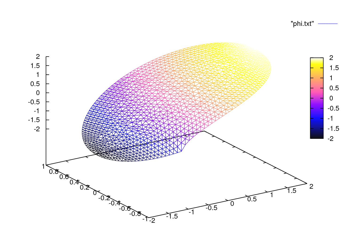
../_images/gnumembrane.png — Fig. 7 The 3D version drawn by `gnuplot` from a file generated by **FreeFEM**

Still that may not take you where you want. Here is an interface with gnuplot (see : web site link ) to produce the Fig. 7.

//to build a gnuplot data file
{
    ofstream ff("graph.txt");
    for (int i = 0; i < Th.nt; i++)
    {
        for (int j = 0; j < 3; j++)
            ff << Th[i][j].x << " "<< Th[i][j].y << " " << phi[][Vh(i,j)] << endl;

        ff << Th[i][0].x << " " << Th[i][0].y << " " << phi[][Vh(i,0)] << "\n\n\n"
    }
}

We use the finite element numbering, where Wh(i,j) is the global index of \(j^{Th}\) degrees of freedom of triangle number \(i\).

Then open gnuplot and do:

set palette rgbformulae 30,31,32
splot "graph.txt" w l pal

This works with P2 and P1, but not with P1nc because the three first degrees of freedom of P1 or P2 are on vertices and not with P1nc.

Here you can use the search bar to search in all FreeFEM examples instead

The list of all matching examples on the right is updated for each new query

Clicking on a search hit or on an example on the right brings up the corresponding script from GitHub

You can also filter the list on the right by selecting one or more intersecting categories on the left tree

Membrane