Misc
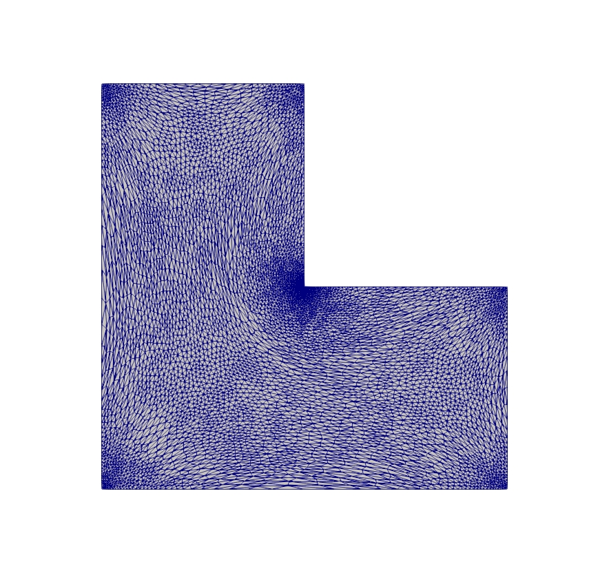
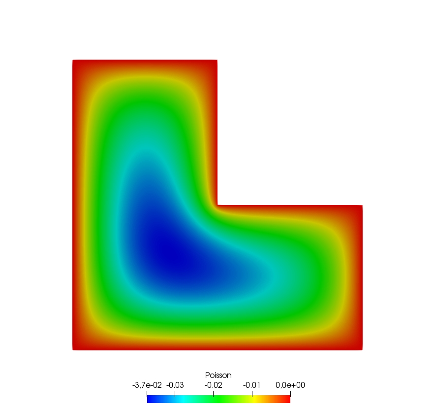
Poisson’s Equation
 1// Parameters
 2int nn = 20;
 3real L = 1.;
 4real H = 1.;
 5real l = 0.5;
 6real h = 0.5;
 7
 8func f = 1.;
 9func g = 0.;
10
11int NAdapt = 10;
12
13// Mesh
14border b1(t=0, L){x=t; y=0;};
15border b2(t=0, h){x=L; y=t;};
16border b3(t=L, l){x=t; y=h;};
17border b4(t=h, H){x=l; y=t;};
18border b5(t=l, 0){x=t; y=H;};
19border b6(t=H, 0){x=0; y=t;};
20
21mesh Th = buildmesh(b1(nn*L) + b2(nn*h) + b3(nn*(L-l)) + b4(nn*(H-h)) + b5(nn*l) + b6(nn*H));
22
23// Fespace
24fespace Vh(Th, P1); // Change P1 to P2 to test P2 finite element
25Vh u, v;
26
27// Macro
28macro grad(u) [dx(u), dy(u)] //
29
30// Problem
31problem Poisson (u, v, solver=CG, eps=-1.e-6)
32   = int2d(Th)(
33        grad(u)' * grad(v)
34   )
35   + int2d(Th)(
36        f * v
37   )
38   + on(b1, b2, b3, b4, b5, b6, u=g)
39   ;
40
41// Mesh adaptation iterations
42real error = 0.1;
43real coef = 0.1^(1./5.);
44for (int i = 0; i < NAdapt; i++){
45   // Solve
46   Poisson;
47
48   // Plot
49   plot(Th, u);
50
51   // Adaptmesh
52   Th = adaptmesh(Th, u, inquire=1, err=error);
53   error = error * coef;
54}
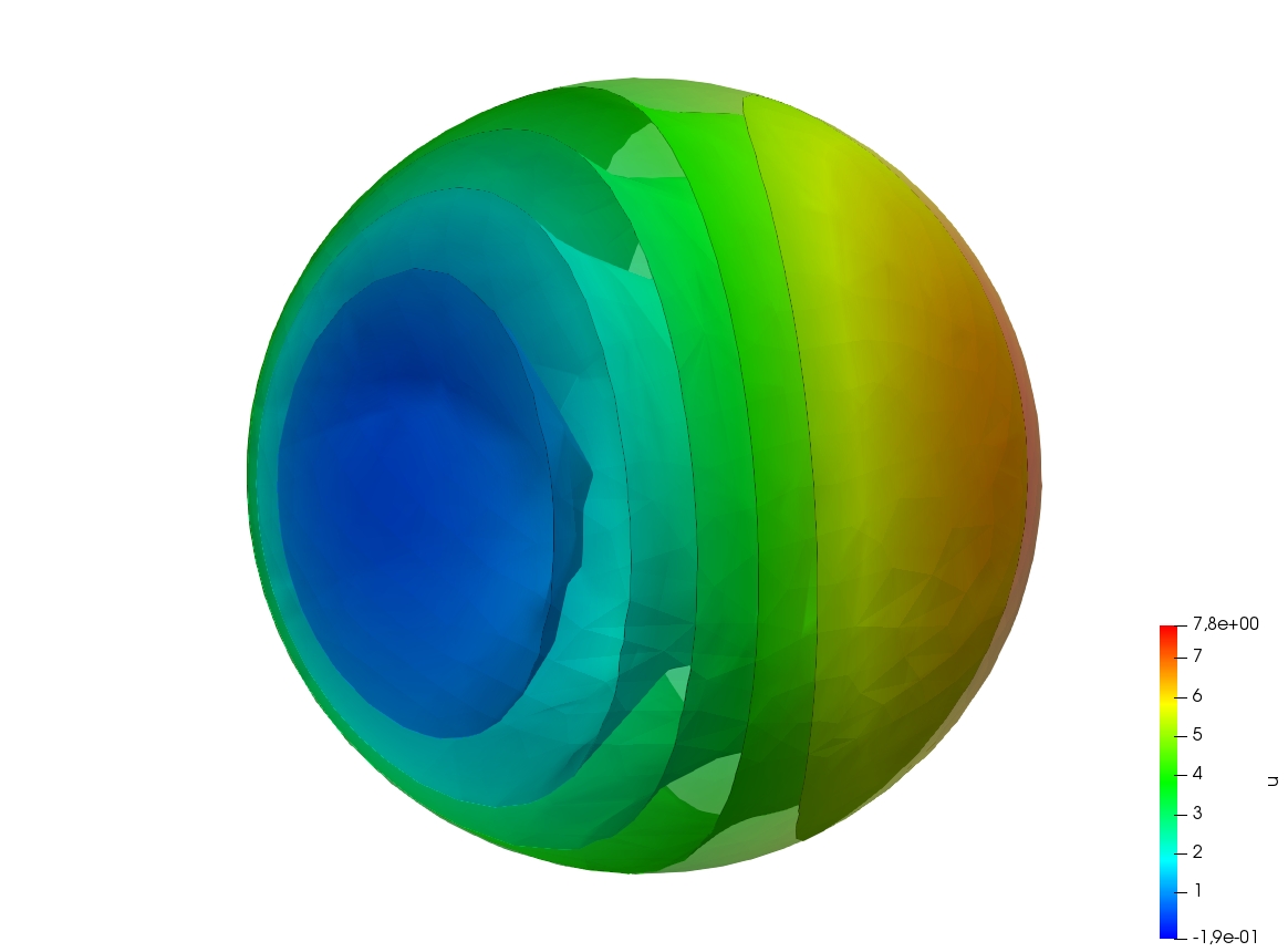
Poisson’s equation 3D
 1load "tetgen"
 2
 3// Parameters
 4real hh = 0.1;
 5func ue = 2.*x*x + 3.*y*y + 4.*z*z + 5.*x*y + 6.*x*z + 1.;
 6func f= -18.;
 7
 8// Mesh
 9mesh Th = square(10, 20, [x*pi-pi/2, 2*y*pi]); // ]-pi/2, pi/2[X]0,2pi[
10func f1 = cos(x)*cos(y);
11func f2 = cos(x)*sin(y);
12func f3 = sin(x);
13func f1x = sin(x)*cos(y);
14func f1y = -cos(x)*sin(y);
15func f2x = -sin(x)*sin(y);
16func f2y = cos(x)*cos(y);
17func f3x = cos(x);
18func f3y = 0;
19func m11 = f1x^2 + f2x^2 + f3x^2;
20func m21 = f1x*f1y + f2x*f2y + f3x*f3y;
21func m22 = f1y^2 + f2y^2 + f3y^2;
22func perio = [[4, y], [2, y], [1, x], [3, x]];
23real vv = 1/square(hh);
24Th = adaptmesh(Th, m11*vv, m21*vv, m22*vv, IsMetric=1, periodic=perio);
25Th = adaptmesh(Th, m11*vv, m21*vv, m22*vv, IsMetric=1, periodic=perio);
26plot(Th);
27
28real[int] domain = [0., 0., 0., 1, 0.01];
29mesh3 Th3 = tetgtransfo(Th, transfo=[f1, f2, f3], nbofregions=1, regionlist=domain);
30plot(Th3);
31
32border cc(t=0, 2*pi){x=cos(t); y=sin(t); label=1;}
33mesh Th2 = buildmesh(cc(50));
34
35// Fespace
36fespace Vh(Th3, P23d);
37Vh u, v;
38Vh uhe = ue;
39cout << "uhe min: " << uhe[].min << " - max: " << uhe[].max << endl;
40cout << uhe(0.,0.,0.) << endl;
41
42fespace Vh2(Th2, P2);
43Vh2 u2, u2e;
44
45// Macro
46macro Grad3(u) [dx(u), dy(u), dz(u)] //
47
48// Problem
49problem Lap3d (u, v, solver=CG)
50    = int3d(Th3)(
51          Grad3(v)' * Grad3(u)
52    )
53    - int3d(Th3)(
54          f * v
55    )
56    + on(0, 1, u=ue)
57    ;
58
59// Solve
60Lap3d;
61cout << "u min: " << u[]. min << " - max: " << u[].max << endl;
62
63// Error
64real err = int3d(Th3)(square(u-ue));
65cout << int3d(Th3)(1.) << " = " << Th3.measure << endl;
66Vh d = ue - u;
67cout << " err = " << err << " - diff l^intfy = " << d[].linfty << endl;
68
69// Plot
70u2 = u;
71u2e = ue;
72plot(u2, wait=true);
73plot(u2, u2e,wait=true);
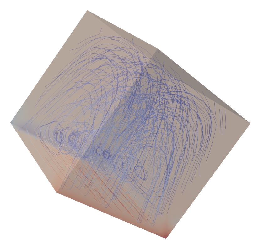
Stokes Equation on a cube
 1load "msh3"
 2load "medit" // Dynamically loaded tools for 3D
 3
 4// Parameters
 5int nn = 8;
 6
 7// Mesh
 8mesh Th0 = square(nn, nn);
 9int[int] rup = [0, 2];
10int[int] rdown = [0, 1];
11int[int] rmid = [1, 1, 2, 1, 3, 1, 4, 1];
12real zmin = 0, zmax = 1;
13mesh3 Th = buildlayers(Th0, nn, zbound=[zmin, zmax],
14    reffacemid=rmid, reffaceup=rup, reffacelow=rdown);
15
16medit("c8x8x8", Th); // 3D mesh visualization with medit
17
18// Fespaces
19fespace Vh2(Th0, P2);
20Vh2 ux, uz, p2;
21
22fespace VVh(Th, [P2, P2, P2, P1]);
23VVh [u1, u2, u3, p];
24VVh [v1, v2, v3, q];
25
26// Macro
27macro Grad(u) [dx(u), dy(u), dz(u)] //
28macro div(u1,u2,u3) (dx(u1) + dy(u2) + dz(u3)) //
29
30// Problem (directly solved)
31solve vStokes ([u1, u2, u3, p], [v1, v2, v3, q])
32    = int3d(Th, qforder=3)(
33          Grad(u1)' * Grad(v1)
34        + Grad(u2)' * Grad(v2)
35        + Grad(u3)' * Grad(v3)
36        - div(u1, u2, u3) * q
37        - div(v1, v2, v3) * p
38        + 1e-10 * q * p
39    )
40    + on(2, u1=1., u2=0, u3=0)
41    + on(1, u1=0, u2=0, u3=0)
42    ;
43
44// Plot
45plot(p, wait=1, nbiso=5); // 3D visualization of pressure isolines
46
47// See 10 plan of the velocity in 2D
48for(int i = 1; i < 10; i++){
49    // Cut plane
50    real yy = i/10.;
51    // 3D to 2D interpolation
52    ux = u1(x,yy,y);
53    uz = u3(x,yy,y);
54    p2 = p(x,yy,y);
55    // Plot
56    plot([ux, uz], p2, cmm="cut y = "+yy, wait= 1);
57}

Cavity
 1//Parameters
 2int m = 300;
 3real L = 1;
 4real rho = 500.;
 5real mu = 0.1;
 6
 7real uin = 1;
 8func fx = 0;
 9func fy = 0;
10int[int] noslip = [1, 2, 4];
11int[int] inflow = [3];
12
13real dt = 0.1;
14real T = 50;
15
16real eps = 1e-3;
17
18//Macros
19macro div(u) (dx(u#x) + dy(u#y))//
20macro grad(u) [dx(u), dy(u)]//
21macro Grad(u) [grad(u#x), grad(u#y)]//
22
23//Time
24real cpu;
25real tabcpu;
26
27//mesh
28border C1(t = 0, L){ x = t; y = 0; label = 1; }
29border C2(t = 0, L){ x = L; y = t; label = 2; }
30border C3(t = 0, L){ x = L-t; y = L; label = 3; }
31border C4(t = 0, L){ x = 0; y = L-t; label = 4; }
32mesh th = buildmesh( C1(m) + C2(m) + C3(m) + C4(m) );
33
34fespace UPh(th, [P2,P2,P1]);
35UPh [ux, uy, p];
36UPh [uhx, uhy, ph];
37UPh [upx, upy, pp];
38
39//Solve
40varf navierstokes([ux, uy, p], [uhx, uhy, ph])
41  = int2d(th)(
42      rho/dt* [ux, uy]'* [uhx, uhy]
43    + mu* (Grad(u):Grad(uh))
44    - p* div(uh)
45    - ph* div(u)
46    - 1e-10 *p*ph
47    )
48
49  + int2d(th) (
50      [fx, fy]' * [uhx, uhy]
51    + rho/dt* [convect([upx, upy], -dt, upx), convect([upx, upy], -dt, upy)]'* [uhx, uhy]
52    )
53
54  + on(noslip, ux=0, uy=0)
55  + on(inflow, ux=uin, uy=0)
56  ;
57
58//Initialization
59[ux, uy, p]=[0, 0, 0];
60
61matrix<real> NS = navierstokes(UPh, UPh, solver=sparsesolver);
62real[int] NSrhs = navierstokes(0, UPh);
63
64//Time loop
65for(int j = 0; j < T/dt; j++){
66  [upx, upy, pp]=[ux, uy, p];
67
68  NSrhs = navierstokes(0, UPh);
69  ux[] = NS^-1 * NSrhs;
70
71  plot( [ux,uy], p, wait=0, cmm=j);
72}
73
74//CPU
75cout << " CPU = " << clock()-cpu << endl ;
76tabcpu = clock()-cpu;