Heat Exchanger
Summary: Here we shall learn more about geometry input and triangulation files, as well as read and write operations.
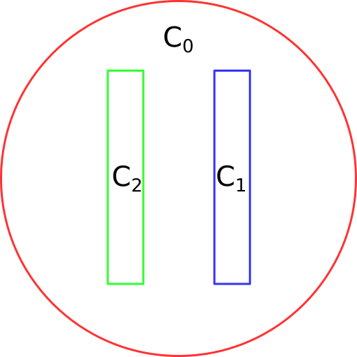
The problem Let \(\{C_{i}\}_{1,2}\), be 2 thermal conductors within an enclosure \(C_0\) (see Fig. 8).
The first one is held at a constant temperature \({u} _{1}\) the other one has a given thermal conductivity \(\kappa_2\) 3 times larger than the one of \(C_0\).
We assume that the border of enclosure \(C_0\) is held at temperature \(20^\circ C\) and that we have waited long enough for thermal equilibrium.
In order to know \({u} (x)\) at any point \(x\) of the domain \(\Omega\), we must solve:
where \(\Omega\) is the interior of \(C_0\) minus the conductor \(C_1\) and \(\Gamma\) is the boundary of \(\Omega\), that is \(C_0\cup C_1\).
Here \(g\) is any function of \(x\) equal to \({u}_i\) on \(C_i\).
The second equation is a reduced form for:
The variational formulation for this problem is in the subspace \(H^1_0(\Omega) \subset H^1(\Omega)\) of functions which have zero traces on \(\Gamma\).
Let us assume that \(C_0\) is a circle of radius 5 centered at the origin, \(C_i\) are rectangles, \(C_1\) being at the constant temperature \(u_1=60^\circ C\) (so we can only consider its boundary).
1// Parameters
2int C1=99;
3int C2=98; //could be anything such that !=0 and C1!=C2
4
5// Mesh
6border C0(t=0., 2.*pi){x=5.*cos(t); y=5.*sin(t);}
7
8border C11(t=0., 1.){x=1.+t; y=3.; label=C1;}
9border C12(t=0., 1.){x=2.; y=3.-6.*t; label=C1;}
10border C13(t=0., 1.){x=2.-t; y=-3.; label=C1;}
11border C14(t=0., 1.){x=1.; y=-3.+6.*t; label=C1;}
12
13border C21(t=0., 1.){x=-2.+t; y=3.; label=C2;}
14border C22(t=0., 1.){x=-1.; y=3.-6.*t; label=C2;}
15border C23(t=0., 1.){x=-1.-t; y=-3.; label=C2;}
16border C24(t=0., 1.){x=-2.; y=-3.+6.*t; label=C2;}
17
18plot( C0(50) //to see the border of the domain
19 + C11(5)+C12(20)+C13(5)+C14(20)
20 + C21(-5)+C22(-20)+C23(-5)+C24(-20),
21 wait=true, ps="heatexb.eps");
22
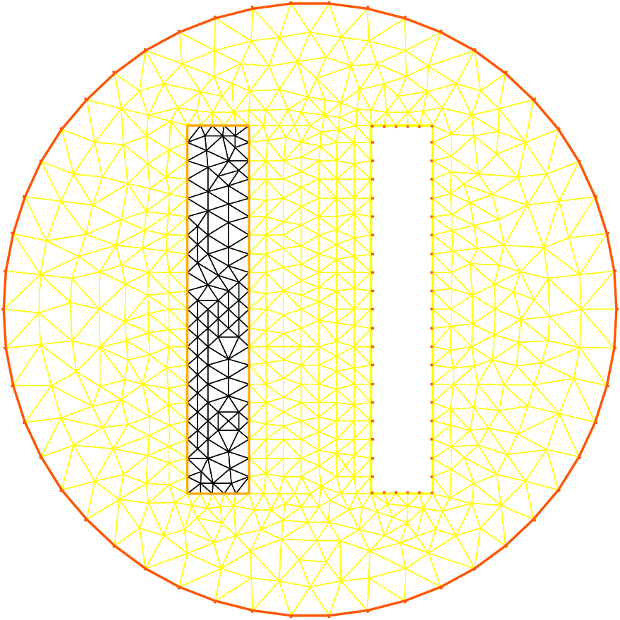
23mesh Th=buildmesh(C0(50)
24 + C11(5)+C12(20)+C13(5)+C14(20)
25 + C21(-5)+C22(-20)+C23(-5)+C24(-20));
26
27plot(Th,wait=1);
28
29// Fespace
30fespace Vh(Th, P1);
31Vh u, v;
32Vh kappa=1 + 2*(x<-1)*(x>-2)*(y<3)*(y>-3);
33
34// Solve
35solve a(u, v)
36 = int2d(Th)(
37 kappa*(
38 dx(u)*dx(v)
39 + dy(u)*dy(v)
40 )
41 )
42 +on(C0, u=20)
43 +on(C1, u=60)
44 ;
45
46// Plot
47plot(u, wait=true, value=true, fill=true, ps="HeatExchanger.eps");
Note the following:
C0is oriented counterclockwise by \(t\), whileC1is oriented clockwise andC2is oriented counterclockwise. This is whyC1is viewed as a hole bybuildmesh.C1andC2are built by joining pieces of straight lines. To group them in the same logical unit to input the boundary conditions in a readable way we assigned a label on the boundaries. As said earlier, borders have an internal number corresponding to their order in the program (check it by adding acout << C22;above). This is essential to understand how a mesh can be output to a file and re-read (see below).As usual the mesh density is controlled by the number of vertices assigned to each boundary. It is not possible to change the (uniform) distribution of vertices but a piece of boundary can always be cut in two or more parts, for instance
C12could be replaced byC121+C122:
1// border C12(t=0.,1.){x=2.; y=3.-6.*t; label=C1;}
2border C121(t=0.,0.7){x=2.; y=3.-6.*t; label=C1;}
3border C122(t=0.7,1.){x=2.; y=3.-6.*t; label=C1;}
4...
5buildmesh(.../*+ C12(20) */ + C121(12) + C122(8) + ...);

Tip
Exercise :
Use the symmetry of the problem with respect to the x axes.
Triangulate only one half of the domain, and set homogeneous Neumann conditions on the horizontal axis.
Writing and reading triangulation files Suppose that at the end of the previous program we added the line
1savemesh(Th, "condensor.msh");
and then later on we write a similar program but we wish to read the mesh from that file. Then this is how the condenser should be computed:
 1// Mesh
 2mesh Sh = readmesh("condensor.msh");
 3
 4// Fespace
 5fespace Wh(Sh, P1);
 6Wh us, vs;
 7
 8// Solve
 9solve b(us, vs)
10    = int2d(Sh)(
11          dx(us)*dx(vs)
12        + dy(us)*dy(vs)
13    )
14    +on(1, us=0)
15    +on(99, us=1)
16    +on(98, us=-1)
17    ;
18
19// Plot
20plot(us);
Note that the names of the boundaries are lost but either their internal number (in the case of C0) or their label number (for C1 and C2) are kept.