Pure Convection : The Rotating Hill

Summary: Here we will present two methods for upwinding for the simplest convection problem. We will learn about Characteristics-Galerkin and Discontinuous-Galerkin Finite Element Methods.

Let \(\Omega\) be the unit disk centered at \((0,0)\); consider the rotation vector field

\[\mathbf{u} = [u1,u2], \qquad u_1 = y,\quad u_2 = -x\]

Pure convection by \(\mathbf{u}\) is

\[\begin{split}\begin{array}{rcl} \partial_t c + \mathbf{u}.\nabla c &= 0 &\hbox{ in } \Omega\times(0,T)\\ c (t=0) &= c ^0 &\hbox{ in } \Omega. \end{array}\end{split}\]

The exact solution \(c(x_t,t)\) at time \(t\) en point \(x_t\) is given by:

\[c(x_t,t)=c^0(x,0)\]

where \(x_t\) is the particle path in the flow starting at point \(x\) at time \(0\). So \(x_t\) are solutions of

\[\dot{x_t} = u(x_t), \quad\ x_{t=0} =x , \quad\mbox{where}\quad \dot{x_t} = \frac{\text{d} ( x_t }{\text{d} t}\]

The ODE are reversible and we want the solution at point \(x\) at time \(t\) ( not at point \(x_t\)) the initial point is \(x_{-t}\), and we have

\[c(x,t)=c^0(x_{-t},0)\]

The game consists in solving the equation until \(T=2\pi\), that is for a full revolution and to compare the final solution with the initial one; they should be equal.

Solution by a Characteristics-Galerkin Method

In FreeFEM there is an operator called convect([u1,u2], dt, c) which compute \(c\circ X\) with \(X\) is the convect field defined by \(X(x)= x_{dt}\) and where \(x_\tau\) is particule path in the steady state velocity field \(\mathbf{u}=[u1,u2]\) starting at point \(x\) at time \(\tau=0\), so \(x_\tau\) is solution of the following ODE:

\[\dot{x}_\tau = u(x_\tau), {x}_{\tau=0}=x.\]

When \(\mathbf{u}\) is piecewise constant; this is possible because \(x_\tau\) is then a polygonal curve which can be computed exactly and the solution exists always when \(\mathbf{u}\) is divergence free; convect returns \(c(x_{df})=C\circ X\).

// Parameters
real dt = 0.17;

// Mesh
border C(t=0., 2.*pi) {x=cos(t); y=sin(t);};
mesh Th = buildmesh(C(100));

// Fespace
fespace Uh(Th, P1);
Uh cold, c = exp(-10*((x-0.3)^2 +(y-0.3)^2));
Uh u1 = y, u2 = -x;

// Time loop
real t = 0;
for (int m = 0; m < 2.*pi/dt; m++){
    t += dt;
    cold = c;
    c = convect([u1, u2], -dt, cold);
    plot(c, cmm=" t="+t +", min="+c[].min+", max="+c[].max);
}

Note

3D plots can be done by adding the qualifyer dim=3 to the plot instruction.

The method is very powerful but has two limitations:

it is not conservative
it may diverge in rare cases when \(|\mathbf{u}|\) is too small due to quadrature error.

Solution by Discontinuous-Galerkin FEM

Discontinuous Galerkin methods take advantage of the discontinuities of \(c\) at the edges to build upwinding. There are may formulations possible. We shall implement here the so-called dual-\(P_1^{DC}\) formulation (see [ERN2006]):

\[\int_\Omega(\frac{c^{n+1}-c^n}{\delta t} +u\cdot\nabla c)w +\int_E(\alpha|n\cdot u|-\frac 12 n\cdot u)[c]w =\int_{E_\Gamma^-}|n\cdot u| cw~~~\forall w\]

where \(E\) is the set of inner edges and \(E_\Gamma^-\) is the set of boundary edges where \(u\cdot n<0\) (in our case there is no such edges). Finally \([c]\) is the jump of \(c\) across an edge with the convention that \(c^+\) refers to the value on the right of the oriented edge.

// Parameters
real al=0.5;
real dt = 0.05;

// Mesh
border C(t=0., 2.*pi) {x=cos(t); y=sin(t);};
mesh Th = buildmesh(C(100));

// Fespace
fespace Vh(Th,P1dc);
Vh w, ccold, v1 = y, v2 = -x, cc = exp(-10*((x-0.3)^2 +(y-0.3)^2));

// Macro
macro n() (N.x*v1 + N.y*v2) // Macro without parameter

// Problem
problem Adual(cc, w)
    = int2d(Th)(
          (cc/dt+(v1*dx(cc)+v2*dy(cc)))*w
    )
    + intalledges(Th)(
          (1-nTonEdge)*w*(al*abs(n)-n/2)*jump(cc)
    )
    - int2d(Th)(
          ccold*w/dt
    )
    ;

// Time iterations
for (real t = 0.; t < 2.*pi; t += dt){
    ccold = cc;
    Adual;
    plot(cc, fill=1, cmm="t="+t+", min="+cc[].min+", max="+ cc[].max);
}

// Plot
real [int] viso = [-0.2, -0.1, 0., 0.1, 0.2, 0.3, 0.4, 0.5, 0.6, 0.7, 0.8, 0.9, 1., 1.1];
plot(cc, wait=1, fill=1, ps="ConvectCG.eps", viso=viso);
plot(cc, wait=1, fill=1, ps="ConvectDG.eps", viso=viso);

Note

New keywords: intalledges to integrate on all edges of all triangles

\[\mathtt{intalledges}(\mathtt{Th}) \equiv \sum_{T\in\mathtt{Th}}\int_{\partial T }\]

(so all internal edges are see two times), nTonEdge which is one if the triangle has a boundary edge and two otherwise, jump to implement \([c]\).

Results of both methods are shown on Fig. 17 nad Fig. 18 with identical levels for the level line; this is done with the plot-modifier viso.

Notice also the macro where the parameter \(\mathbf{u}\) is not used (but the syntax needs one) and which ends with a //; it simply replaces the name n by (N.x*v1+N.y*v2). As easily guessed N.x,N.y is the normal to the edge.

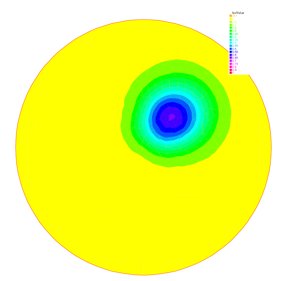
convectCG — Fig. 17 The rotating hill after one revolution with Characteristics-Galerkin

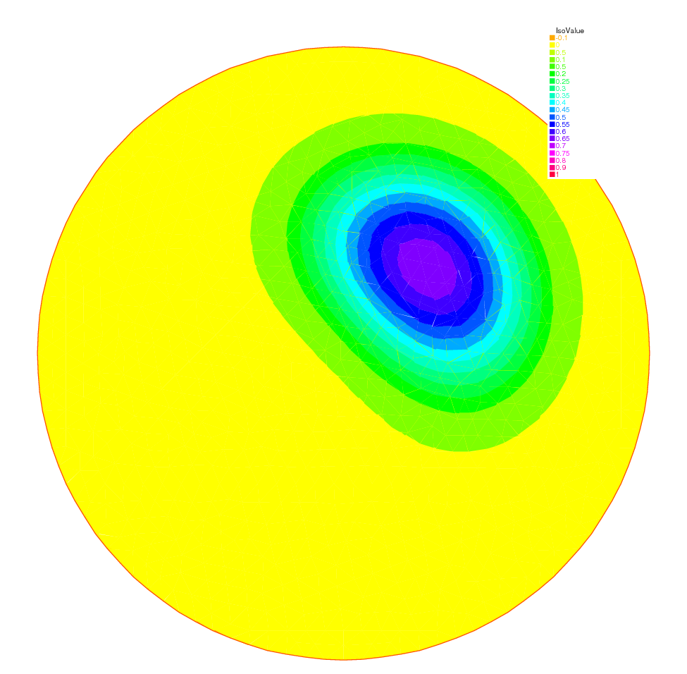
convectDG — Fig. 18 The rotating hill after one revolution with Discontinuous \(P_1\) Galerkin

Rotating hill

Now if you think that DG is too slow try this:

// Mesh
border C(t=0., 2.*pi) {x=cos(t); y=sin(t);};
mesh Th = buildmesh(C(100));

fespace Vh(Th,P1);//P1,P2,P0,P1dc,P2dc, uncond stable

Vh vh,vo,u1 = y, u2 = -x, v = exp(-10*((x-0.3)^2 +(y-0.3)^2));
real dt = 0.03,t=0, tmax=2*pi, al=0.5, alp=200;

problem  A(v,vh) = int2d(Th)(v*vh/dt-v*(u1*dx(vh)+u2*dy(vh)))
  + intalledges(Th)(vh*(mean(v)*(N.x*u1+N.y*u2)
                   +alp*jump(v)*abs(N.x*u1+N.y*u2)))
  + int1d(Th,1)(((N.x*u1+N.y*u2)>0)*(N.x*u1+N.y*u2)*v*vh)
  - int2d(Th)(vo*vh/dt);

varf  Adual(v,vh) = int2d(Th)((v/dt+(u1*dx(v)+u2*dy(v)))*vh)
  + intalledges(Th)((1-nTonEdge)*vh*(al*abs(N.x*u1+N.y*u2)
                             -(N.x*u1+N.y*u2)/2)*jump(v));

varf rhs(vo,vh)= int2d(Th)(vo*vh/dt);

real[int] viso=[-0.1,0,0.1,0.2,0.3,0.4,0.5,0.6,0.7,0.8,0.9,1,1.1];

matrix AA=Adual(Vh,Vh,solver=GMRES);
matrix BB=rhs(Vh,Vh);

for ( t=0; t< tmax ; t+=dt)
{
   vo[]=v[];
   vh[]=BB*vo[];
   v[]=AA^-1*vh[];
   plot(v,fill=0,viso=viso,cmm=" t="+t + ", min=" + v[].min + ", max=" +  v[].max);
};

Here you can use the search bar to search in all FreeFEM examples instead

The list of all matching examples on the right is updated for each new query

Clicking on a search hit or on an example on the right brings up the corresponding script from GitHub

You can also filter the list on the right by selecting one or more intersecting categories on the left tree

Pure Convection : The Rotating Hill

Solution by a Characteristics-Galerkin Method

Solution by Discontinuous-Galerkin FEM