Visualization
Results created by the finite element method can be a huge set of data, so it is very important to render them easy to grasp.
There are two ways of visualization in FreeFEM:
One, the default view, which supports the drawing of meshes, isovalues of real FE-functions, and of vector fields, all by the command
plot(see Plot section below). For publishing purpose, FreeFEM can store these plots as postscript files.Another method is to use external tools, for example, gnuplot (see Gnuplot section, medit section, Paraview section, Matlab/Octave section) using the command
systemto launch them and/or to save the data in text files.
Plot
With the command plot, meshes, isovalues of scalar functions, and vector fields can be displayed.
The parameters of the plot command can be meshes, real FE functions, arrays of 2 real FE functions, arrays of two double arrays, to plot respectively a mesh, a function, a vector field, or a curve defined by the two double arrays.
Note
The length of an arrow is always bound to be in [5‰, 5%] of the screen size in order to see something.
The plot command parameters are listed in the Reference part.
The keyboard shortcuts are:
enter tries to show plot
p previous plot (10 plots saved)
? shows this help
+,- zooms in/out around the cursor 3/2 times
= resets the view
r refreshes plot
up, down, left, right special keys to tanslate
3 switches 3d/2d plot keys :
z,Z focal zoom and zoom out
H,h increases or decreases the Z scale of the plot
mouse motion:
left button rotates
right button zooms (ctrl+button on mac)
right button +alt tanslates (alt+ctrl+button on mac)
a,A increases or decreases the arrow size
B switches between showing the border meshes or not
i,I updates or not: the min/max bound of the functions to the window
n,N decreases or increases the number of iso value arrays
b switches between black and white or color plotting
g switches between grey or color plotting
f switches between filling iso or iso line
l switches between lighting or not
v switches between show or not showing the numerical value of colors
m switches between show or not showing the meshes
w window dump in file ffglutXXXX.ppm
* keep/drop viewpoint for next plot
k complex data / change view type
ESC closes the graphics process before version 3.22, after no way to close
otherwise does nothing
For example:
 1real[int] xx(10), yy(10);
 2
 3mesh Th = square(5,5);
 4
 5fespace Vh(Th, P1);
 6
 7//plot scalar and vectorial FE function
 8Vh uh=x*x+y*y, vh=-y^2+x^2;
 9plot(Th, uh, [uh, vh], value=true, ps="three.eps", wait=true);
10
11//zoom on box defined by the two corner points [0.1,0.2] and [0.5,0.6]
12plot(uh, [uh, vh], bb=[[0.1, 0.2], [0.5, 0.6]],
13   wait=true, grey=true, fill=true, value=true, ps="threeg.eps");
14
15//compute a cut
16for (int i = 0; i < 10; i++){
17   x = i/10.;
18   y = i/10.;
19   xx[i] = i;
20   yy[i] = uh; //value of uh at point (i/10., i/10.)
21}
22plot([xx, yy], ps="likegnu.eps", wait=true);
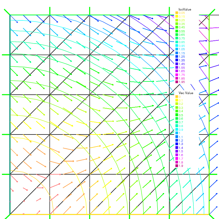
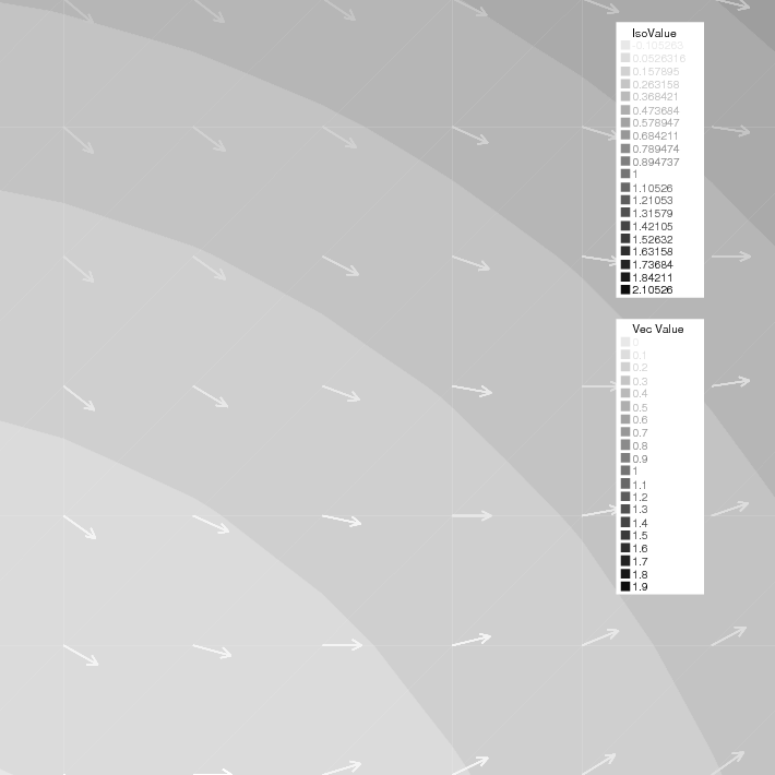
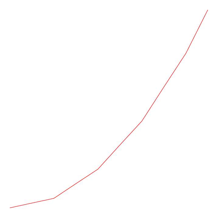
Fig. 114 Plots a cut of uh. Note that a refinement of the same can be obtained in combination with gnuplot
Plot
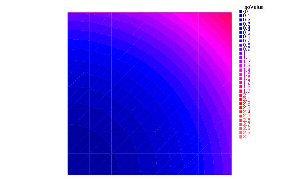
To change the color table and to choose the value of iso line you can do:
1// from: \url{http://en.wikipedia.org/wiki/HSV_color_space}
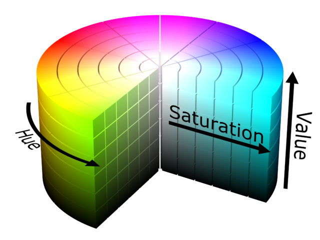
2// The HSV (Hue, Saturation, Value) model defines a color space
3// in terms of three constituent components:
4// HSV color space as a color wheel
5// Hue, the color type (such as red, blue, or yellow):
6// Ranges from 0-360 (but normalized to 0-100% in some applications, like here)
7// Saturation, the "vibrancy" of the color: Ranges from 0-100%
8// The lower the saturation of a color, the more "grayness" is present
9// and the more faded the color will appear.
10// Value, the brightness of the color: Ranges from 0-100%
11
12mesh Th = square(10, 10, [2*x-1, 2*y-1]);
13
14fespace Vh(Th, P1);
15Vh uh=2-x*x-y*y;
16
17real[int] colorhsv=[ // color hsv model
18 4./6., 1 , 0.5, // dark blue
19 4./6., 1 , 1, // blue
20 5./6., 1 , 1, // magenta
21 1, 1. , 1, // red
22 1, 0.5 , 1 // light red
23 ];
24 real[int] viso(31);
25
26 for (int i = 0; i < viso.n; i++)
27 viso[i] = i*0.1;
28
29 plot(uh, viso=viso(0:viso.n-1), value=true, fill=true, wait=true, hsv=colorhsv);
Note
See HSV example for the complete script.
Link with gnuplot
Example Membrane shows how to generate a gnuplot from a FreeFEM file. Here is another technique which has the advantage of being online, i.e. one doesn’t need to quit FreeFEM to generate a gnuplot.
However, this works only if gnuplot is installed, and only on an Unix-like computer.
Add to the previous example:
1{// file for gnuplot
2   ofstream gnu("plot.gp");
3   for (int i = 0; i < n; i++)
4      gnu << xx[i] << " " << yy[i] << endl;
5}
6
7// to call gnuplot command and wait 5 second (due to the Unix command)
8// and make postscript plot
9exec("echo 'plot \"plot.gp\" w l \n pause 5 \n set term postscript \n set output \"gnuplot.eps\" \n replot \n quit' | gnuplot");

Note
See Plot example for the complete script.
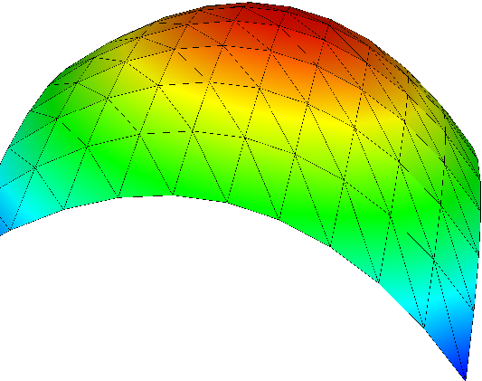
Link with medit
As said above, medit is a freeware display package by Pascal Frey using OpenGL. Then you may run the following example.
Now medit software is included in FreeFEM under ffmedit name.
The medit command parameters are listed in the Reference part.
With version 3.2 or later
1load "medit"
2
3mesh Th = square(10, 10, [2*x-1, 2*y-1]);
4
5fespace Vh(Th, P1);
6Vh u=2-x*x-y*y;
7
8medit("u", Th, u);
Before:
 1mesh Th = square(10, 10, [2*x-1, 2*y-1]);
 2
 3fespace Vh(Th, P1);
 4Vh u=2-x*x-y*y;
 5
 6savemesh(Th, "u", [x, y, u*.5]); //save u.points and u.faces file
 7// build a u.bb file for medit
 8{
 9   ofstream file("u.bb");
10   file << "2 1 1 " << u[].n << " 2 \n";
11   for (int j = 0; j < u[].n; j++)
12      file << u[][j] << endl;
13}
14//call medit command
15exec("ffmedit u");
16//clean files on unix-like OS
17exec("rm u.bb u.faces u.points");
Note
See Medit example for the complete script.
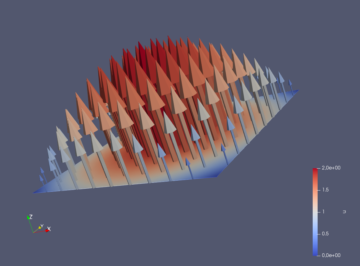
Link with Paraview
One can also export mesh or results in the .vtk format in order to post-process data using Paraview.
 1load "iovtk"
 2
 3mesh Th = square(10, 10, [2*x-1, 2*y-1]);
 4
 5fespace Vh(Th, P1);
 6Vh u=2-x*x-y*y;
 7
 8int[int] Order = [1];
 9string DataName = "u";
10savevtk("u.vtu", Th, u, dataname=DataName, order=Order);
Warning
Finite element variables saved using paraview must be in P0 or P1
Note
See Paraview example for the complete script.
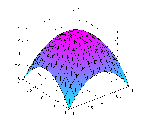
Link with Matlab© and Octave
In order to create a plot from a FreeFEM simulation in Octave and Matlab the mesh, the finite element space connectivity and the simulation data must be written to files:
1include "ffmatlib.idp"
2
3mesh Th = square(10, 10, [2*x-1, 2*y-1]);
4fespace Vh(Th, P1);
5Vh u=2-x*x-y*y;
6
7savemesh(Th,"export_mesh.msh");
8ffSaveVh(Th,Vh,"export_vh.txt");
9ffSaveData(u,"export_data.txt");
Within Matlab or Octave the files can be plot with the ffmatlib library:
1addpath('path to ffmatlib');
2[p,b,t]=ffreadmesh('export_mesh.msh');
3vh=ffreaddata('export_vh.txt');
4u=ffreaddata('export_data.txt');
5ffpdeplot(p,b,t,'VhSeq',vh,'XYData',u,'ZStyle','continuous','Mesh','on');
6grid;
Note
For more Matlab / Octave plot examples have a look at the tutorial section Matlab / Octave Examples or visit the ffmatlib library on github.