Getting started

For a given function \(f(x,y)\), find a function \(u(x,y)\) satisfying :

(1)\[\begin{split}\begin{array}{rcl} -\Delta u(x,y) &= f(x,y) & \mbox{ for all }(x,y)\mbox{ in }\Omega\\ u(x,y) &= 0 & \mbox{ for all }(x,y)\mbox{ on }\partial\Omega \end{array}\end{split}\]

Here \(\partial\Omega\) is the boundary of the bounded open set \(\Omega\subset\mathbb{R}^2\) and \(\Delta u = \frac{\partial^2 u}{\partial x^2 } + \frac{\partial^2 u}{\partial y^2}\).

We will compute \(u\) with \(f(x,y)=xy\) and \(\Omega\) the unit disk. The boundary \(C=\partial\Omega\) is defined as:

\[C=\{(x,y)|\; x=\cos(t),\, y=\sin(t),\, 0\le t\le 2\pi\}\]

Note

In FreeFEM, the domain \(\Omega\) is assumed to be described by the left side of its boundary.

The following is the FreeFEM program which computes \(u\):

// Define mesh boundary
border C(t=0, 2*pi){x=cos(t); y=sin(t);}

// The triangulated domain Th is on the left side of its boundary
mesh Th = buildmesh(C(50));

// The finite element space defined over Th is called here Vh
fespace Vh(Th, P1);
Vh u, v;// Define u and v as piecewise-P1 continuous functions

// Define a function f
func f= x*y;

// Get the clock in second
real cpu=clock();

// Define the PDE
solve Poisson(u, v, solver=LU)
    = int2d(Th)(    // The bilinear part
          dx(u)*dx(v)
        + dy(u)*dy(v)
    )
    - int2d(Th)(    // The right hand side
          f*v
    )
    + on(C, u=0);   // The Dirichlet boundary condition

// Plot the result
plot(u);

// Display the total computational time
cout << "CPU time = " << (clock()-cpu) << endl;

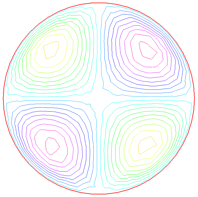
As illustrated in Fig. 2, we can see the isovalue of \(u\) by using FreeFEM plot command (see line 29 above).

firstTh — Fig. 1 Mesh Th by `buildmesh(C(50))`

Poisson’s equation

Note

The qualifier solver=LU (line 18) is not required and by default a multi-frontal LU is used.

The lines containing clock are equally not required.

Tip

Note how close to the mathematics FreeFEM language is.

Lines 19 to 24 correspond to the mathematical variational equation:

\[\int_{T_h} ( \frac{\partial u}{\partial x}\frac{\partial v}{\partial x} + \frac{\partial u}{\partial y}\frac{\partial v}{\partial y} )\text{d} x \text{d} y = \int_{T_h}f v\text{d} x\text{d} y\]

for all \(v\) which are in the finite element space \(V_h\) and zero on the boundary \(C\).

Tip

Change P1 into P2 and run the program.

This first example shows how FreeFEM executes with no effort all the usual steps required by the finite element method (FEM). Let’s go through them one by one.

On the line 2:

The boundary \(\Gamma\) is described analytically by a parametric equation for \(x\) and for \(y\). When \(\Gamma=\sum_{j=0}^J \Gamma_j\) then each curve \(\Gamma_j\) must be specified and crossings of \(\Gamma_j\) are not allowed except at end points.

The keyword label can be added to define a group of boundaries for later use (boundary conditions for instance). Hence the circle could also have been described as two half circle with the same label:

border Gamma1(t=0, pi){x=cos(t); y=sin(t); label=C};
border Gamma2(t=pi, 2.*pi){x=cos(t); y=sin(t); label=C};

Boundaries can be referred to either by name (Gamma1 for example) or by label (C here) or even by its internal number here 1 for the first half circle and 2 for the second (more examples are in Meshing Examples).

On the line 5

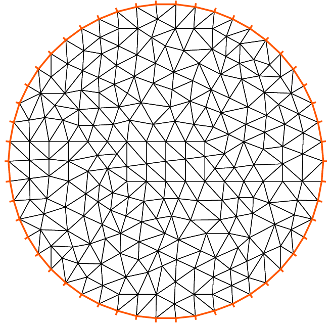
The triangulation \(\mathcal{T}_h\) of \(\Omega\) is automatically generated by buildmesh(C(50)) using 50 points on C as in Fig. 1.

The domain is assumed to be on the left side of the boundary which is implicitly oriented by the parametrization. So an elliptic hole can be added by typing:

border C(t=2.*pi, 0){x=0.1+0.3*cos(t); y=0.5*sin(t);};

If by mistake one had written:

border C(t=0, 2.*pi){x=0.1+0.3*cos(t); y=0.5*sin(t);};

then the inside of the ellipse would be triangulated as well as the outside.

Note

Automatic mesh generation is based on the Delaunay-Voronoi algorithm. Refinement of the mesh are done by increasing the number of points on \(\Gamma\), for example buildmesh(C(100)), because inner vertices are determined by the density of points on the boundary.

Mesh adaptation can be performed also against a given function f by calling adaptmesh(Th,f).

Now the name \(\mathcal{T}_h\) (Th in FreeFEM) refers to the family \(\{T_k\}_{k=1,\cdots,n_t}\) of triangles shown in Fig. 1.

Traditionally \(h\) refers to the mesh size, \(n_t\) to the number of triangles in \(\mathcal{T}_h\) and \(n_v\) to the number of vertices, but it is seldom that we will have to use them explicitly.

If \(\Omega\) is not a polygonal domain, a “skin” remains between the exact domain \(\Omega\) and its approximation \(\Omega_h=\cup_{k=1}^{n_t}T_k\). However, we notice that all corners of \(\Gamma_h = \partial\Omega_h\) are on \(\Gamma\).

On line 8:

A finite element space is, usually, a space of polynomial functions on elements, triangles here only, with certain matching properties at edges, vertices etc. Here fespace Vh(Th, P1) defines \(V_h\) to be the space of continuous functions which are affine in \(x,y\) on each triangle of \(T_h\).

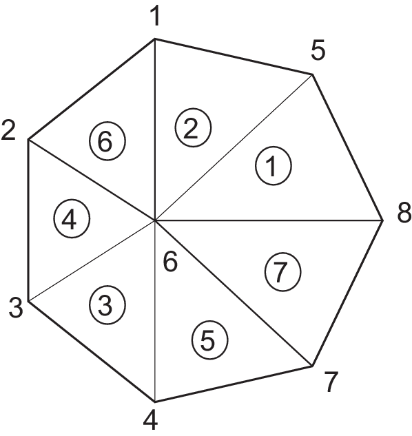
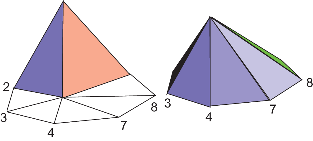
As it is a linear vector space of finite dimension, basis can be found. The canonical basis is made of functions, called the hat function \(\phi_k\), which are continuous piecewise affine and are equal to 1 on one vertex and 0 on all others. A typical hat function is shown on Fig. 4.

Hat functions

Note

The easiest way to define \(\phi_k\) is by making use of the barycentric coordinates \(\lambda_i(x,y),~i=1,2,3\) of a point \(q=(x,y)\in T\), defined by \(\sum_i\lambda_i=1,~~~\sum_i\lambda_i\vec q^i=\vec q\) where \(q^i,~i=1,2,3\) are the 3 vertices of \(T\). Then it is easy to see that the restriction of \(\phi_k\) on \(T\) is precisely \(\lambda_k\).

Then:

(2)\[V_h(\mathcal{T}_h,P_1)=\left\{w(x,y)\left|\; w(x,y)=\sum_{k=1}^{M}w_k\phi_k(x,y),\, w_k\textrm{ are real numbers}\right.\right\}\]

where \(M\) is the dimension of \(V_h\), i.e. the number of vertices. The \(w_k\) are called the degrees of freedom of \(w\) and \(M\) the number of degree of freedom.

It is said also that the nodes of this finite element method are the vertices.

Setting the problem

On line 9, Vh u, v declares that \(u\) and \(v\) are approximated as above, namely:

(3)\[u(x,y)\simeq u_h(x,y)=\sum_{k=0}^{M-1} u_k\phi_k(x,y)\]

On the line 12, the right hand side f is defined analytically using the keyword func.

Line 18 to 26 define the bilinear form of equation (1) and its Dirichlet boundary conditions.

This variational formulation is derived by multiplying (1) by \(v(x,y)\) and integrating the result over \(\Omega\):

\[-\int_{\Omega}v\Delta u \,\text{d} x\text{d} y = \int_{\Omega} vf\, \text{d} x\text{d} y\]

Then, by Green’s formula, the problem is converted into finding \(u\) such that

\[a(u,v) - \ell(f,v) = 0 \quad \forall v \mbox{ satisfying }v=0\mbox{ on }\partial\Omega.\]

with:

(4)\[\begin{split}\begin{array}{rcl} a(u,v) &=& \int_{\Omega}\nabla u\cdot \nabla v \,\text{d} x\text{d} y\\ \ell(f,v) &=& \int_{\Omega}fv\, \text{d} x\text{d} y \end{array}\end{split}\]

In FreeFEM the Poisson problem can be declared only as in:

Vh u,v; problem Poisson(u,v) = ...

and solved later as in:

Poisson; //the problem is solved here

or declared and solved at the same time as in:

Vh u,v; solve Poisson(u,v) = ...

and (4) is written with dx(u) \(=\partial u/\partial x\), dy(u) \(=\partial u/\partial y\) and:

\(\displaystyle{\int_{\Omega}\nabla u\cdot \nabla v\, \text{d} x\text{d} y \longrightarrow}\) int2d(Th)( dx(u)*dx(v) + dy(u)*dy(v) )

\(\displaystyle{\int_{\Omega}fv\, \text{d} x\text{d} y \longrightarrow}\) int2d(Th)( f*v ) (Notice here, \(u\) is unused)

Warning

In FreeFEM bilinear terms and linear terms should not be under the same integral indeed to construct the linear systems FreeFEM finds out which integral contributes to the bilinear form by checking if both terms, the unknown (here u) and test functions (here v) are present.

Solution and visualization

On line 15, the current time in seconds is stored into the real-valued variable cpu.

Line 18, the problem is solved.

Line 29, the visualization is done as illustrated in Fig. 2.

(see Plot for zoom, postscript and other commands).

Line 32, the computing time (not counting graphics) is written on the console. Notice the C++-like syntax; the user needs not study C++ for using FreeFEM, but it helps to guess what is allowed in the language.

Access to matrices and vectors

Internally FreeFEM will solve a linear system of the type

(5)\[\sum_{j=0}^{M-1} A_{ij}u_j - F_i=0 ,\quad i=0,\cdots,M-1;\qquad F_i=\int_{\Omega}f\phi_i\, \text{d} x\text{d} y\]

which is found by using (3) and replacing \(v\) by \(\phi_i\) in (4). The Dirichlet conditions are implemented by penalty, namely by setting \(A_{ii}=10^{30}\) and \(F_i=10^{30}*0\) if \(i\) is a boundary degree of freedom.

Note

The number \(10^{30}\) is called tgv (très grande valeur or very high value in english) and it is generally possible to change this value, see the item :freefem`solve, tgv=`

The matrix \(A=(A_{ij})\) is called stiffness matrix. If the user wants to access \(A\) directly he can do so by using (see section Variational form, Sparse matrix, PDE data vector for details).

varf a(u,v)
    = int2d(Th)(
          dx(u)*dx(v)
        + dy(u)*dy(v)
    )
    + on(C, u=0)
    ;
matrix A = a(Vh, Vh); //stiffness matrix

The vector \(F\) in (5) can also be constructed manually:

varf l(unused,v)
    = int2d(Th)(
          f*v
    )
    + on(C, unused=0)
    ;
Vh F;
F[] = l(0,Vh); //F[] is the vector associated to the function F

The problem can then be solved by:

u[] = A^-1*F[]; //u[] is the vector associated to the function u

Note

Here u and F are finite element function, and u[] and F[] give the array of value associated (u[] \(\equiv (u_i)_{i=0,\dots,M-1}\) and F[] \(\equiv (F_i)_{i=0,\dots,M-1}\)).

So we have:

\[\mathtt{u}(x,y) = \sum_{i=0}^{M-1} \mathtt{u[][}i\mathtt{]} \phi_i(x,y) , \qquad \mathtt{F}(x,y) = \sum_{i=0}^{M-1} \mathtt{F[][}i\mathtt{]} \phi_i(x,y)\]

where \(\phi_i, i=0...,,M-1\) are the basis functions of Vh like in equation :eq: equation3, and \(M = \mathtt{Vh.ndof}\) is the number of degree of freedom (i.e. the dimension of the space Vh).

The linear system (5) is solved by UMFPACK unless another option is mentioned specifically as in:

Vh u, v;
problem Poisson(u, v, solver=CG) = int2d(...

meaning that Poisson is declared only here and when it is called (by simply writing Poisson;) then (5) will be solved by the Conjugate Gradient method.

Here you can use the search bar to search in all FreeFEM examples instead

The list of all matching examples on the right is updated for each new query

Clicking on a search hit or on an example on the right brings up the corresponding script from GitHub

You can also filter the list on the right by selecting one or more intersecting categories on the left tree

Getting started